High-content behavioral analysis of Caenorhabditis elegans in precise spatiotemporal chemical environments

Abstract

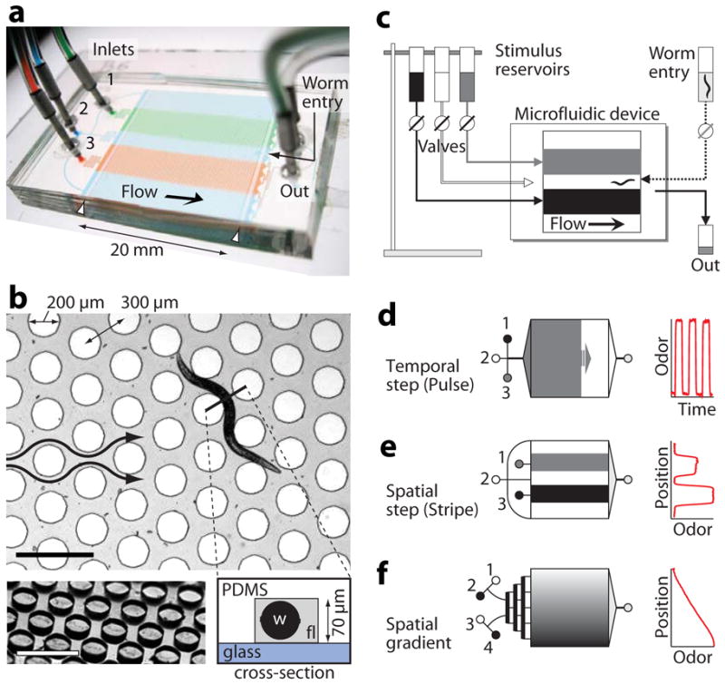
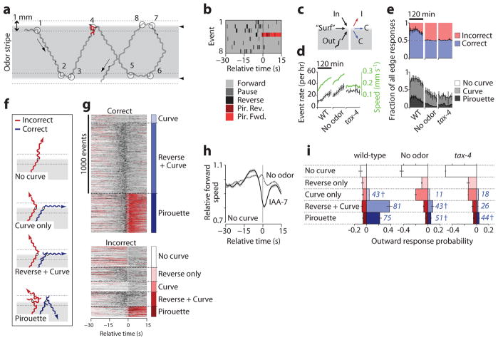
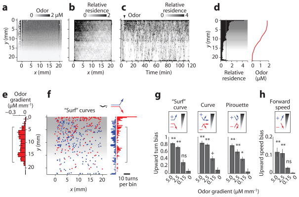
To quantitatively understand chemosensory behaviors, it is desirable to present many animals with repeatable, well-defined chemical stimuli. To that end, we describe a microfluidic system to analyze Caenorhabditis elegans behavior in defined temporal and spatial stimulus patterns. A 2 cm × 2 cm structured arena allowed C. elegans to perform crawling locomotion in a controlled liquid environment. We characterized behavioral responses to attractive odors with three stimulus patterns: temporal pulses, spatial stripes and a linear concentration gradient, all delivered in the fluid phase to eliminate variability associated with air-fluid transitions. Different stimulus configurations preferentially revealed turning dynamics in a biased random walk, directed orientation into an odor stripe and speed regulation by odor. We identified both expected and unexpected responses in wild-type worms and sensory mutants by quantifying dozens of behavioral parameters. The devices are inexpensive, easy to fabricate, reusable and suitable for delivering any liquid-borne stimulus.

Figure 1

Worm behavioral arena and stimulus patterns. (a) Photo of the microfluidic device, configured such that continuous flow of three streams (1–3) produces a stable pattern of dye stripes within the arena. Worm barriers prevent passage out of the arena (white arrowheads). (b) Top view showing arena geometry. A young adult worm crawls through fluid-filled channels (gray) between cylindrical microposts (white circles). Arrows indicate the direction of flow. Bottom left shows an oblique view of the micropost array before device assembly. Bottom right schematic shows a cross-section, indicating the glass bottom surface, PDMS top surface and posts, worm (w) and stimulus fluid (fl). Scale bars, 500 μm. (c) Stimuli flow by gravity from elevated reservoirs through external valves into the device. Worms are loaded with a syringe. (d–f) Upstream channels are tailored to each stimulus pattern: inlet channels converge to a distribution tree for stimulus pulses (d), remain separated for stimulus stripes (e), or pass though a mixing tree to create linear or sigmoidal concentration profiles (f). The graphs on the right show the corresponding odor patterns, estimated by measured dye concentration with respect to time or position in the device.

Figure 2

Locomotory behavior in structured arenas. (a) Representative tracks from a single worm demonstrating the indicated behavioral states. Dot indicates the head of the worm. Arrows and shading show the direction of travel. (b) The path taken by one representative wild-type worm (of 24) over 1 hr shows navigation across the entire buffer-filled arena (above) and a magnified region (below). Color indicates time in the device. Black points indicate the animal centroid at 0.5 s intervals. (c) The centroid path for the animal in b, colored according to behavioral state. Swimming behavior at the upstream and downstream barriers was removed from analysis, and path breaks indicate temporary collisions with other animals. Specific reversal (R) and pirouette (Pir) behaviors are labeled in the magnified view below. (d) The graphs show the timecourse of morphological parameters (green plots, above) and speed (shaded plot, below) for the magnified worm path in c. The corresponding behavioral state (bottom plot, colored as in c) was automatically determined from these parameters for each video frame (Supplementary Notes); for example, reversals are bounded by high angular velocity, and omega turns are identified by high aspect ratio and sharp reorientation (dashed lines). Labeled events correspond to the behavior trace in c. Scale bars, 500 μm (a and b, lower panel) and 2 mm (b, upper panel).

Figure 3

Odor pulse assay. (a) Odor concentration estimated from dye absorbance during one cycle of IAA pulses (top), and corresponding instantaneous forward locomotion speed (bottom, n = 48 worms) are shown. (b) Ethogram showing the instantaneous behavioral state of animals subjected to the odor pattern in a. Each row represents one animal, and four 15-min cycles are shown stacked for a total of 192 rows. Speed traces and ethograms for each animal were aligned in time to the odor step it experienced. (c) Instantaneous behavioral state probability from b, excluding collisions and animals near the barriers. (d) Initiation of individual omega turns from b (black points, top) and average omega turn rate per animal (below, mean ± s.d.). (e) Average stimulus (top graph) and behavioral dynamics (lower graphs) for repeated odor removals (shading indicates 95% confidence for odor and s.e.m. for state probability, n = 24 pulses). Peak response times (arrows) are indicated. The dotted lines show buffer-buffer control switches. (f) Average probability of response to odor addition and removal (mean ± s.e.m., n = 6–24 pulses). Numbers indicate percent probability. *, P < 0.01 vs. wild-type odor-free probability of forward (gray), reverse (black), or pirouette (red) responses. (g) Ethogram showing a ±10 s window around odor removal #24 (black box in b), sorted by the predominant behavioral state after odor removal. (h) Responses of 23 individual animals to 24 repeated odor removal steps, colored as in g. *, P < 0.05; ns, not significant vs. the population mean by the mass function of the trinomial distribution and the Benjamini–Hochberg–Yekutieli correction for false discovery rate.

Figure 4

Odor stripe assay. (a) The image shows the arena with two odor stripes containing 0.92 or 1.84 μM IAA and dye, surrounded by buffer. (b) Relative x-y residence of 24 worms over 80 min (a value of 1 represents a uniform distribution). (c) Timecourse of worm residence along the y-axis over time, with odor added at 3 min (arrowhead). (d) Histograms of residence relative to different spatial odor patterns (red plots above and shading below). (e) Heatmaps of wild-type, mutant, and rescued animal residence in odor or buffer stripes over time, as in c. (f) Spatially-averaged behavioral parameters within 1.8 mm surrounding each odor edge (arrowhead), as described in Supplementary Fig. 9. Shading indicates odor. Directional parameters are shown for animals traveling downward before the event, with the upper (green) and lower (black) plots representing inward and outward movement relative to odor, respectively. Dot indicates worm head, and event locations correspond to the animal centroid at event initiation (circle). Data are mean ± s.e.m., n = 2–10 experiments for turn rates, n = 8–24 odor edges for other parameters, averaged over 37–230 animals per condition. (g) Spatial plot and histogram of upward (blue) and downward (red) “surf” curves occurring within 0.5 mm of the odor edge (dotted lines), by 25 worms over 1 hr. (h) Top, mean chemotaxis (CTX) index from 20–80 min, defined as (animal density in odor – density out of odor)/(total density); below, peak outward forward speed relative to speed in odor. Error bars as in f, with significance assessed by ANOVA and Bonferroni’s correction for multiple comparisons. **, P < 0.001; * P < 0.01; ns, not significant compared with wild-type no-odor control.

Figure 5

Turning responses at sharp spatial odor gradients. (a) A wild-type worm track within a 0.92 μM IAA odor stripe (gray) shows turning events (circled) initiated within 0.5 mm of the odor edge (dotted lines) or odor edge crossings. (b) Ethogram shows –30 s to +15 s relative to the eight numbered edge encounter events in a. (c) Events were grouped according to the direction of edge approach (inward, “surfing” (horizontal), or outward) and by the response outcome (correctly remaining in the odor (C), or incorrectly leaving the odor (I)). All eight events in a,b are correct. (d) Outward edge event rates (black) for wild-type experiments with odor (WT) or buffer stripes (No odor) and tax-4 with odor over 120 min, and average forward speed (green). (e) Correctness (above) and type (below) of all edge-triggered responses over 120 min. (f) Representative wild-type worm paths shown for correct and incorrect outward responses. Shading indicates odor. (g) Behavior rasters for wild-type worms heading outward, grouped by correctness and response category, n = 2,208 responses from 159 worms over 80 min. (h) Relative forward speed for WT animals that did not pirouette, curve or reverse upon exit of odor or buffer stripes. (i) Probabilities of outward responses for worms exiting odor and buffer stripes, indicating the percent correct for each category in blue. Data are mean ± s.e.m., n = 2–10 experiments. † indicates no significant difference from random (50% correct), P > 0.2 via two-tailed t-test.

Figure 6

Odor gradient assay. (a) Odor concentration gradient from 0–1.84 μM IAA in the arena, visualized with dye. (b) Relative x-y residence of 25 worms tracked over 120 min in the gradient; (a value of 1 represents a uniform distribution). (c) Timecourse of worm residence in the odor gradient, established at 5 min (arrowhead). (d) Distribution of wild-type worms over 120 min (average of 5 experiments) subjected to a spatial odor gradient (red plot and gray shading). (e) Odor concentration gradient calculated from odor profile in d (mean ± s.d., n = 6 points per 1.67 mm wide y-bin). (f) Location in the arena of “surf” curves directed up (blue) or down (red) the odor gradient. Bracket marks the region of constant odor gradient analyzed for turning bias. (g) Relative prevalence of “surf” curves, other curves, and pirouettes directed up (+1, blue) or down (–1, red) odor gradients from 0–5 μM mm⁻¹ IAA. Indices on the y axis are defined as (# events up–# events down)/(total events per y-bin) averaged over the gradient region (bracketed in e, f). Bars indicate mean ± s.e.m., n = 5–9 y-bins averaged over 2–10 experiments. **, p<0.001; *, p<0.01; ns, not significant compared with wild-type no-odor control. Data for sharp gradients (≥2.5 μM mm⁻¹) were obtained with stripe device (Fig. 4). (h) Upward bias of forward speed, defined as (speed up gradient–speed down gradient)/(mean speed per y-bin); statistics as in g.

References

1. Robinson DA. The use of control systems analysis in the neurophysiology of eye movements. Annu Rev Neurosci. 1981;4:463–503. - PubMed
1. Branson K, Robie AA, Bender J, Perona P, Dickinson MH. High-throughput ethomics in large groups of Drosophila. Nat Methods. 2009;6:451–7. - PMC - PubMed
1. Ward S. Chemotaxis by the nematode Caenorhabditis elegans: identification of attractants and analysis of the response by use of mutants. Proc Natl Acad Sci U S A. 1973;70:817–21. - PMC - PubMed
1. Bargmann CI, Hartwieg E, Horvitz HR. Odorant-selective genes and neurons mediate olfaction in C. elegans. Cell. 1993;74:515–27. - PubMed
1. Chalasani SH, et al. Dissecting a circuit for olfactory behaviour in Caenorhabditis elegans. Nature. 2007;450:63–70. - PubMed
Publication types