Climate related sea-level variations over the past two millennia

Abstract

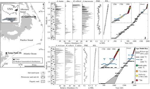
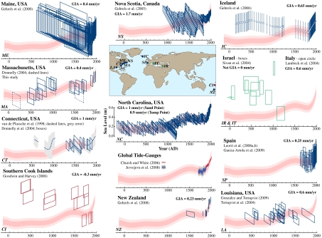
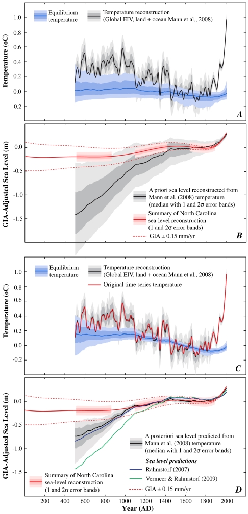
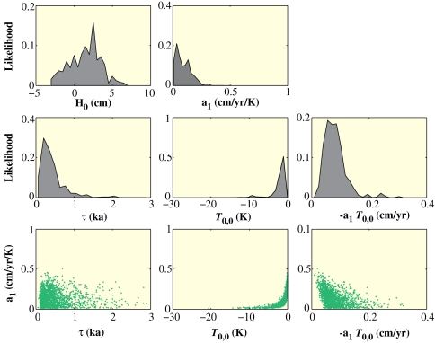
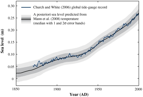
We present new sea-level reconstructions for the past 2100 y based on salt-marsh sedimentary sequences from the US Atlantic coast. The data from North Carolina reveal four phases of persistent sea-level change after correction for glacial isostatic adjustment. Sea level was stable from at least BC 100 until AD 950. Sea level then increased for 400 y at a rate of 0.6 mm/y, followed by a further period of stable, or slightly falling, sea level that persisted until the late 19th century. Since then, sea level has risen at an average rate of 2.1 mm/y, representing the steepest century-scale increase of the past two millennia. This rate was initiated between AD 1865 and 1892. Using an extended semiempirical modeling approach, we show that these sea-level changes are consistent with global temperature for at least the past millennium.

Fig. 1.

Litho-, bio-, and chrono-stratigraphy of the Sand Point (A) and Tump Point (B) cores (North Carolina, USA). Chronologies were developed using AMS ¹⁴C dating (conventional, high-precision, HP, and bomb-spike), ²¹⁰Pb, ¹³⁷Cs, and a pollen horizon (Ambrosia). All dating results were combined to produce a probabilistic age-depth model for each core (10), shown as a gray-shaded area (95% confidence limits). This model estimated the age (with unique uncertainty) of samples at 1 cm resolution. Paleo marsh elevation (PME) above mean sea-level (MSL) was estimated for each sample by application of transfer functions to complete foraminiferal assemblages. Only the most abundant species are shown (). RSL was estimated by subtracting PME from measured sample altitude.

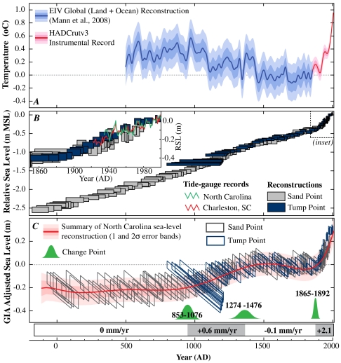
Fig. 2.

(A) Composite EIV global land plus ocean global temperature reconstruction (1), smoothed with a 30-year LOESS low-pass filter (blue). Data since AD 1850 (red) are HADCrutv3 instrumental temperatures. Values are relative to a preindustrial average for AD 1400–1800 (B) RSL reconstructions at Sand Point and Tump Point since BC 100. Boxes represent sample-specific age and sea-level uncertainties (2σ). Inset is a comparison with nearby tide-gauge data. (C) GIA-adjusted sea level at Sand Point and Tump Point expressed relative to a preindustrial average for AD 1400–1800. Sea-level data points are represented by parallelograms because of distortion caused by GIA, which has a larger effect on the older edge of a data point than on the younger edge. Times of changes in the rate of sea-level rise (95% confidence change-point intervals) are shown. Pink envelope is a nine degree polynomial to visually summarize the North Carolina sea-level reconstruction.

Fig. 3.

Late Holocene sea-level reconstructions after correction for GIA. Rate applied (listed) was taken from the original publication when possible. In Israel, land and ocean basin subsidence had a net effect of zero (26). Reconstructions from salt marshes are shown in blue; archaeological data in green; and coral microatolls in red. Tide-gauge data expressed relative to AD 1950–2000 average, error from (32) in gray. Vertical and horizontal scales for all datasets are the same, and are shown for North Carolina. Datasets were vertically aligned for comparison with the summarized North Carolina reconstruction (pink).

Fig. 4.

A priori and a posteriori sea-level predicted from paleo-temperature data. Temperature and GIA-adjusted sea level are expressed relative to AD 1400–1800 averages. Shaded error bands indicate 1σ and 2σ uncertainties. (A) A priori temperature (gray) and equilibrium temperature (blue). (B) A priori sea level predicted from temperature (gray) and summary of North Carolina sea-level reconstruction as cutaway bands (pink). An additional, systematic, GIA uncertainty (additive linear trend of 0.15 mm/y) is indicated by dashed red lines and exceeds the 2σ uncertainty of estimated GIA (0.1 mm/y). Temperatures and model parameters are set to the a priori distributions (Table S3). (C) A posteriori temperature [gray, original from ref.  is the red line] and equilibrium temperature T₀(t) (blue). (D) Sea level predicted from temperature (gray) with summary of North Carolina sea-level reconstruction (pink). Salt-marsh proxy data used in Bayesian update were down-weighted by a factor of 10 and used only after AD 1000. Sea level predicted from refs.  and are shown for comparison. Dashed red lines are as B.

Fig. 5.

Posterior probability density distributions and correlation point clouds for unknown parameters and functions of interest; ka is thousands of years.

Fig. 6.

Comparison of posterior solution with instrumental (tide gauge) data for AD 1880–2000. Black, gray: predicted sea level based on Mann et al. (1) temperatures (effectively HADcrutv3), as shown in Fig. 4D. Blue: Church and White (31) sea level, corrected for the artificial reservoir storage contribution (4).

References

1. Mann ME, et al. Proxy-based reconstructions of hemispheric and global surface temperature variations over the past two millennia. Proc Nat'l Acad Sci USA. 2008;105:13252–13257. - PMC - PubMed
1. Jansen E, et al. Paleoclimate. In: Solomon S, et al., editors. Climate Change 2007: The Physical Science Basis. Contributionof Working Group I to the Fourth Assessment Report of the Intergovernmental Panel on Climate Change. New York City: Cambridge University Press; 2007.
1. Rahmstorf S. A semi-empirical approach to projecting future sea-level rise. Science. 2007;315:368–370. - PubMed
1. Vermeer M, Rahmstorf S. Global sea level linked to global temperature. Proc Nat'l Acad Sci USA. 2009;106:21527–21532. - PMC - PubMed
1. Horton B, Edwards R. Quantifying Holocene sea-level change using intertidal foraminifera: lessons from the British Isles. Fredericksburg, VA: Cushman Foundation for Foraminiferal Research; 2006. p. 97.
LinkOut - more resources