. 2011 Jun;22(4):553-571.
doi: 10.1002/env.1086.

On the use of a PM(2.5) exposure simulator to explain birthweight

Affiliations

On the use of a PM(2.5) exposure simulator to explain birthweight

Veronica J Berrocal et al. Environmetrics. 2011 Jun.

Abstract

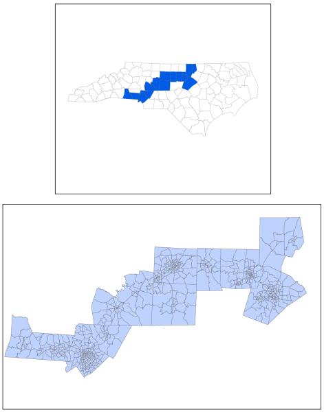
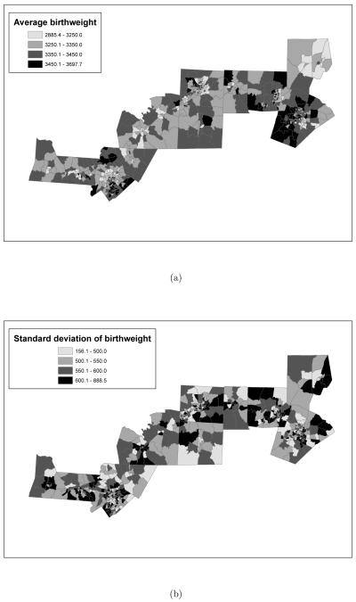
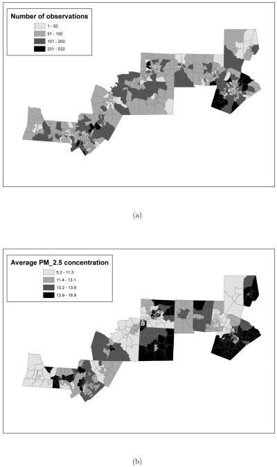
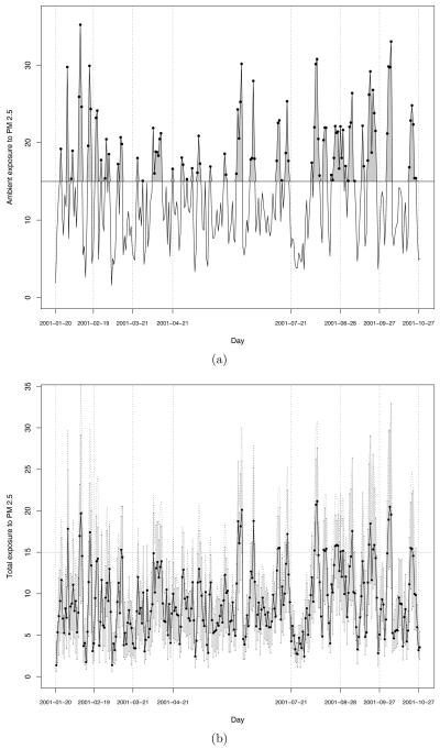
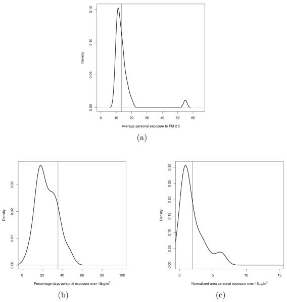
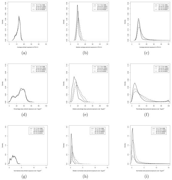
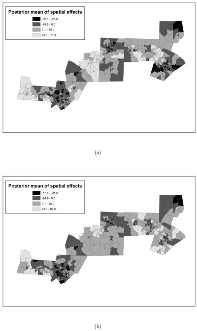
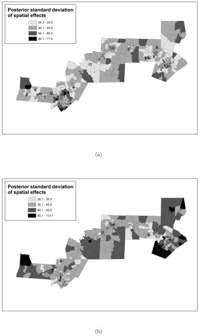
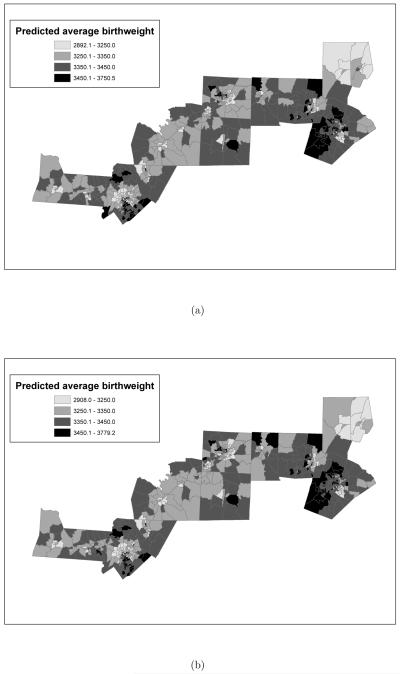
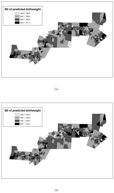
In relating pollution to birth outcomes, maternal exposure has usually been described using monitoring data. Such characterization provides a misrepresentation of exposure as it (i) does not take into account the spatial misalignment between an individual's residence and monitoring sites, and (ii) it ignores the fact that individuals spend most of their time indoors and typically in more than one location. In this paper, we break with previous studies by using a stochastic simulator to describe personal exposure (to particulate matter) and then relate simulated exposures at the individual level to the health outcome (birthweight) rather than aggregating to a selected spatial unit.We propose a hierarchical model that, at the first stage, specifies a linear relationship between birthweight and personal exposure, adjusting for individual risk factors and introduces random spatial effects for the census tract of maternal residence. At the second stage, our hierarchical model specifies the distribution of each individual's personal exposure using the empirical distribution yielded by the stochastic simulator as well as a model for the spatial random effects.We have applied our framework to analyze birthweight data from 14 counties in North Carolina in years 2001 and 2002. We investigate whether there are certain aspects and time windows of exposure that are more detrimental to birthweight by building different exposure metrics which we incorporate, one by one, in our hierarchical model. To assess the difference in relating ambient exposure to birthweight versus personal exposure to birthweight, we compare estimates of the effect of air pollution obtained from hierarchical models that linearly relate ambient exposure and birthweight versus those obtained from our modeling framework.Our analysis does not show a significant effect of PM(2.5) on birthweight for reasons which we discuss. However, our modeling framework serves as a template for analyzing the relationship between personal exposure and longer term health endpoints.


Figures

Figure 1
Figure 1
Fourteen counties in North Carolina included in this analysis (top panel) and, in detail, the census tracts contained in the fourteen counties (bottom panel).
Figure 2
Figure 2
(a) Average birthweight and (b) standard deviation of birthweigth (in grams) by census tract for births that occurred in years 2001 and 2002. In both panels the breakpoints of each class are the quartiles of the variable displayed.
Figure 3
Figure 3
(a) Number of observations per census tract. (b) Average PM2.5 concentration (in μg/m3) by census tract in fourteen counties in North Carolina during years 2001-2002. In panel (b) the breakpoints are the quartiles of the distribution of average concentration.
Figure 4
Figure 4
(a) Ambient exposure curve or daily exposure to “fused” ambient PM2.5 concentration during the entire course of the pregnancy for a woman of living in a census tract in Mecklenburg. (b) Range of the 30 daily personal exposure values associated to the woman in consideration obtained from the SHEDS-PM simulator (gray vertical parallel lines) and median of the 30 daily personal exposure values (black solid line and black dots).
Figure 5
Figure 5
(a) Distributions of the average personal exposure to PM2.5 during the entire pregnancy for the mother considered in Figure 4(a). (b) Distribution of the percentage of days the personal exposure to PM2.5 was above 15 μg/m3 during the entire pregnancy for the mother considered in Figure 4(a). (c) Distributions of the normalized area under the personal exposure curve above 15 μg/m3 during the entire pregnancy for the mother considered in Figure 4(a). In panels (a)-(c) the vertical line display the value of the corresponding three metrics obtained using the ambient exposure.
Figure 6
Figure 6
Kernel density estimate of the distribution of the three metrics considered over the entire pregnancy. (a) Average ambient exposure, (b) median average personal exposure, and (c) average personal exposure; (d) percentage of days ambient exposure was above 15 μg/m3, (e) median percentage of days personal exposure was above 15 μg/m3, and (f) percentage of days personal exposure was above 15 μg/m3; (g) normalized area under ambient exposure curve above 15 μg/m3, (h) median normalized area under personal exposure curve above 15 μg/m3, and (i) normalized area under personal exposure curve above 15 μg/m3. In each panel, the kernel density estimates are grouped by age groups.
Figure 7
Figure 7
Posterior means of the random spatial effects obtained from the model where the exposure metric is: (a) “normalized area ambient exposure curve was above 15μg/m3 versus (b) “normalized area personal exposure curve was above 15μg/m3. In both models, the time window of exposure is the entire pregnancy. Additionally, both posterior means are reported in grams.
Figure 8
Figure 8
Posterior standard deviations of the random spatial effects obtained from the models where the exposure metric is: (a) “normalized area ambient exposure curve was above 15μg/m3 versus (b) “normalized area personal exposure curve was above 15μg/m3. In both models the time window of exposure is the entire pregnancy. Additionally, both posterior standard deviations are reported in grams.
Figure 9
Figure 9
Posterior predictive mean of average birth weight (in grams) by census tract as obtained from the model where the exposure metric is: (a) “normalized area ambient exposure curve was above 15μg/m3 versus (b) “normalized area personal exposure curve was above 15μg/m3. In both models the time window of exposure is the entire pregnancy. Additionally, both posterior predictive means are reported in grams.
Figure 10
Figure 10
Posterior predictive standard deviation of average birth weight (in grams) by census tract as obtained from the model where the exposure metric is: (a) “normalized area ambient exposure curve was above 15μg/m3 versus (b) “normalized area personal exposure curve was above 15μg/m3. Time window of exposure is the course of the entire pregnancy. Additionally, both posterior predictive standard deviations are reported in grams.

References

    1. Armstrong BK, White E, Saracci R. Principles of exposure measurement in epidemiology. Oxford University Press; 1992.
    1. Banerjee S, Carlin BP, Gelfand AE. Hierarchical Modeling and Analysis for Spatial Data. Chapman & Hall/CRC; Boca Raton, Fla: 2004.
    1. Basu R, Woodruff TJ, Parker JD, Saulnier L, Schoendorf KC. Comparing exposure metrics in the relationship between PM2.5 and birth weight in California. Journal of Exposure Analysis and Environmental Epidemiology. 2004;14:391–396. - PubMed
    1. Bell ML, Ebisu K, Belanger K. Ambient air pollution and low birth weight in Connecticut and Massachussetts. Environmental Health Perspectives. 2007;115:1118–1124. - PMC - PubMed
    1. Besag J. Spatial interaction and the statistical analysis of lattice systems. Journal of the Royal Statistical Society Series B. 1974;36:192–236.