Generation of diverse biological forms through combinatorial interactions between tissue polarity and growth

Abstract

A major problem in biology is to understand how complex tissue shapes may arise through growth. In many cases this process involves preferential growth along particular orientations raising the question of how these orientations are specified. One view is that orientations are specified through stresses in the tissue (axiality-based system). Another possibility is that orientations can be specified independently of stresses through molecular signalling (polarity-based system). The axiality-based system has recently been explored through computational modelling. Here we develop and apply a polarity-based system which we call the Growing Polarised Tissue (GPT) framework. Tissue is treated as a continuous material within which regionally expressed factors under genetic control may interact and propagate. Polarity is established by signals that propagate through the tissue and is anchored in regions termed tissue polarity organisers that are also under genetic control. Rates of growth parallel or perpendicular to the local polarity may then be specified through a regulatory network. The resulting growth depends on how specified growth patterns interact within the constraints of mechanically connected tissue. This constraint leads to the emergence of features such as curvature that were not directly specified by the regulatory networks. Resultant growth feeds back to influence spatial arrangements and local orientations of tissue, allowing complex shapes to emerge from simple rules. Moreover, asymmetries may emerge through interactions between polarity fields. We illustrate the value of the GPT-framework for understanding morphogenesis by applying it to a growing Snapdragon flower and indicate how the underlying hypotheses may be tested by computational simulation. We propose that combinatorial intractions between orientations and rates of growth, which are a key feature of polarity-based systems, have been exploited during evolution to generate a range of observed biological shapes.

Figure 1. 2D growth patterns with uniform POL gradient.

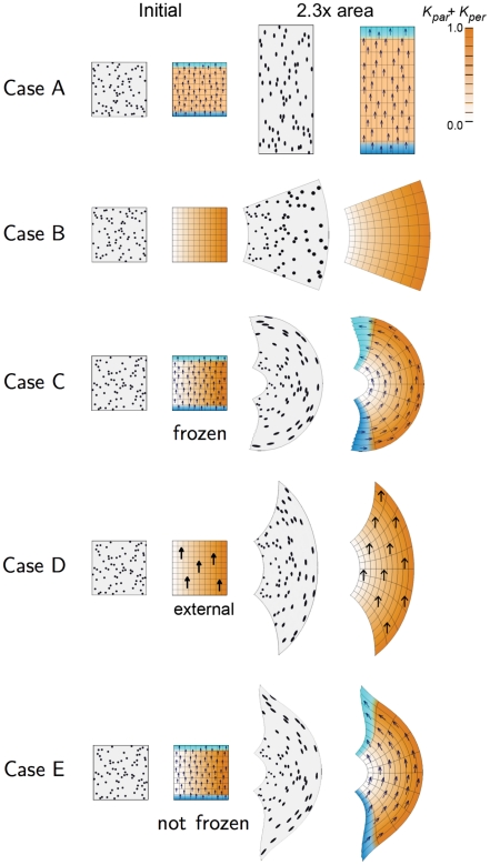
Column 1 shows the initial state drawn with randomly scattered circular marked clones. Column 2 shows the initial state drawn with a regular grid and coloured to show areal specified growth rate (, orange), POL gradient direction (arrows), organiser (dark blue), and organiser (cyan). Columns 3 and 4 show the state after growth for a certain period. In Cases A, C, the POL gradient, once formed is no longer modified through propagation and deforms with the canvas. In Cases D, the POL gradient is held vertically by an external system. In Case E the POL continues to diffuse so the gradient is continually updated as the shape changes during growth. Deformations of the grid can be compared with the transformations of shape described in . (Mesh of 3200 elements, growth magnitudes around 1 per unit time, , runtime min for each example. has arbitrary units.).

Figure 2. 2D growth patterns with non-uniform POL gradient.

Colours and symbols as for Figure 1.

Figure 3. Shapes growing in 3D from a square canvas.

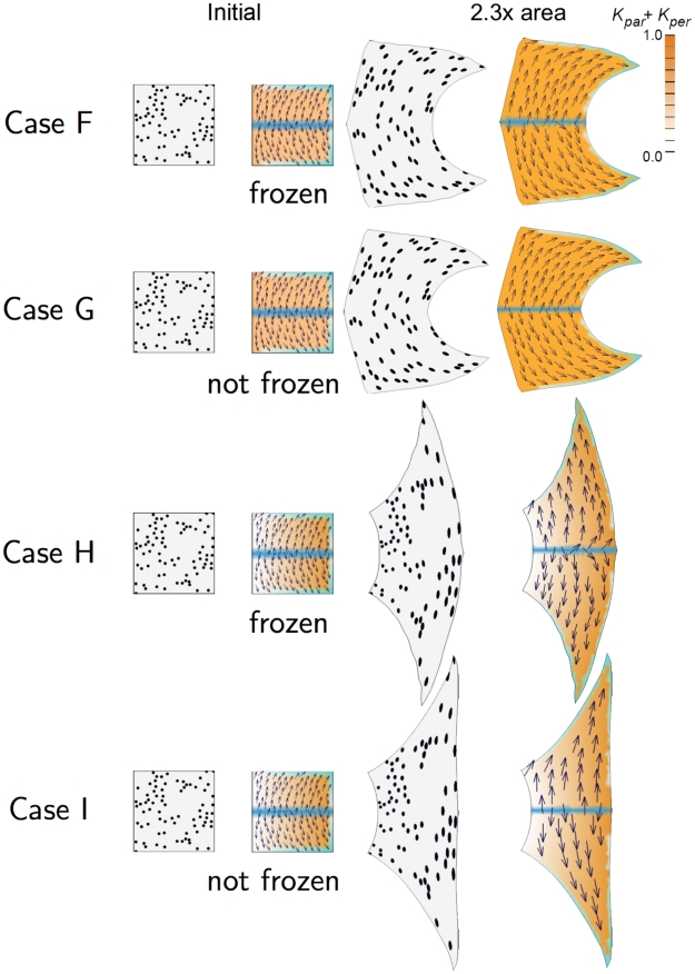
In all cases there is a background specified growth rate (light orange) and each column shows the result of growing to a given multiple of the initial area. Symbols and colour coding as for Figure 1. (Mesh of 1800–2600 elements, growth magnitudes around 1 per unit time, , runtime 5 to 8 min for each example. has arbitrary units.).

Figure 4. Shapes growing in 3D with superimposed gradients of POL.

Symbols, colour coding, and execution parameters as for Figure 3.

Figure 5. Case R: Spatially varying isotropic specified growth rates.

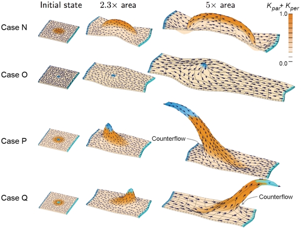
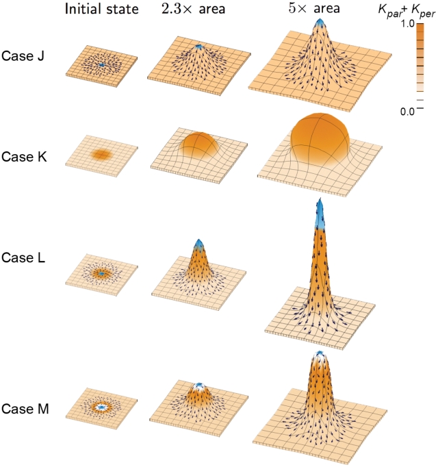
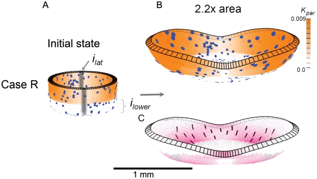
(A) Initial shape with three regions, and . Orange colour denotes the value of specified areal growth. The initially circular discs monitor local shape changes. (B) Shape after growing to 2.2x the area. (C) As (B) but showing regions of resultant anisotropic growth (magenta) and its orientation (lines). (Mesh of 5600 elements, growth magnitudes around 0.018 per unit time, , runtime min for each example. has arbitrary units. Vertices of the base are fixed in the Z-axis.) (A movie of this development is in ‘Video S1’.).

Figure 6. Cases S and T: An initially uniform polarity field with spatially varying anisotropic specified growth rates.

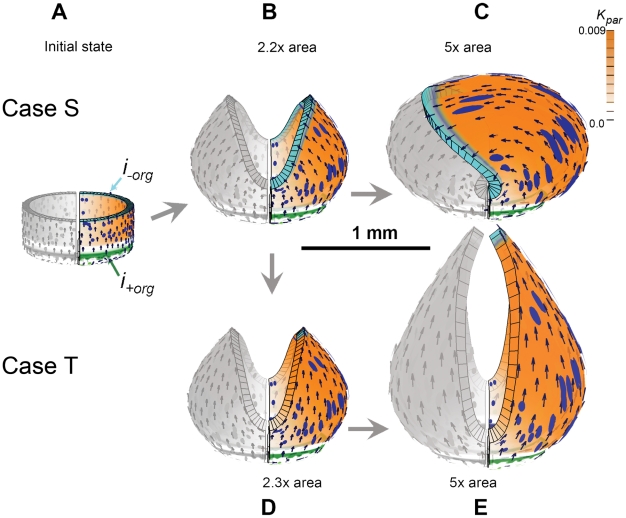
(A) Initial shape with arrows showing proximodistal gradient of POL organised by the green and cyan regions (bottom and top) jonly half of the tube is shown colour-coded. Orange colour denotes the value of . (B) Case S. At 2.2x areal growth the sides are arching over. Blue ellipses (induced as circles in initial state) show regions of local anisotropic growth. (C) Arching continues and at 5x areal growth the two sides overlap (there is no collision detection in our current software). (D) Case T. At 2.2x areal growth the distal organiser (cyan) is spatially redistributed to create two small patches causing the orientation of growth to change (arrows) and growth continues upwards (E). (Mesh of 5600 elements, growth magnitudes around 0.018 per unit time, , runtime min for each example. has arbitrary units. Vertices of the base are fixed in the Z-axis.) (Movies of these developments, C and D, are in ‘Video S2’ and ‘Video S3’.).

Figure 7. Patterns of growth in the Snapdragon model .

(A) Initial canvas showing organisers of polarity, and (green and cyan respectively) and cylindrical shape. Orange indicates growth rate parallel to the POL gradient. (B) By the end of the early growth phase, extra ventral growth (dark orange) creates an arch (as in Figure 6). (C) At the beginning of the late phase is formed and anisotropic growth has reoriented along the new axis (arrows show polariser gradient that now points towards , cyan). (D) Adult shape in which the ventral arch has grown upwards (see Section in Fig.1C). (E) Vertical section through adult shape. (F) Similar view of the same model except that anisotropic growth is not reoriented. (Mesh of 3000 elements, growth magnitudes around 0.003 per unit time, hours, runtime min for each example. has arbitrary units.) (Movies of these developments, B, C, E, F, are in ‘Video S4’, ‘Video S5’, ‘Video S6’, ‘Video S7’.).

Figure 8. Invagination in the developing Drosophila embryo.

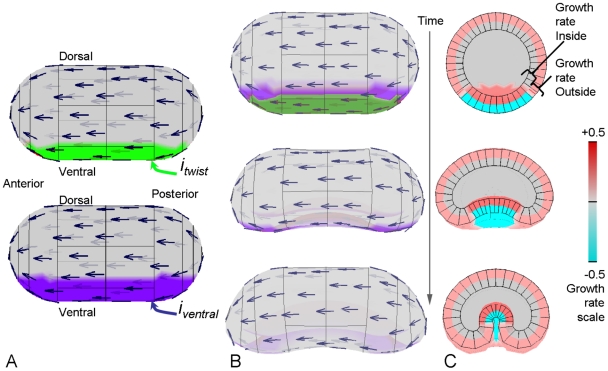
(A) Initial pattern of and on a shape that is polarised from posterior to anterior (arrows). (B) Side view of the developing embryo. The patterns become occluded as the furrow develops. (C) Transverse section of embryo showing colours representing relative specified growth rates perpendicular to the polariser gradient on the internal and external faces. The furrow is produced by a shrinkage on the outside coupled with an expansion on the inside and a net shrinkage in the ventral region (specified by ). Cyan shows negative specified growth on the outside and dark red shows positive growth on the inside. The images are all to the same scale.

Figure 9. Specified and residual strain.

(A) The initial state. (B) Exploded view of the specified growth of each tile, with the original sizes superimposed in grey. (C) The minimum-energy shape that results from the constraint of continuity.

Figure 10. Comparing dissipating residual strains, Cases U and V with accumulating residual strains Cases W and X.

The residual strain after growth is revealed in three ways: by colour (the residual strain is shown in blue); by cutting and re-equilibrating the canvas (Cases U and W); and by releasing constraints (Cases V and X). In Case U growth produces an arc but there is no accumulated strain - no colour - and there is no further change in shape on cutting. Likewise Case V. However, in Case W the shape changes on cutting and in Case X the shape change on releasing constraints. Both these changes reveal the accumulated strains.

Figure 11. Relieving accumulated strain by cutting.

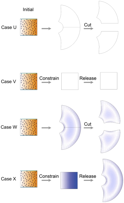
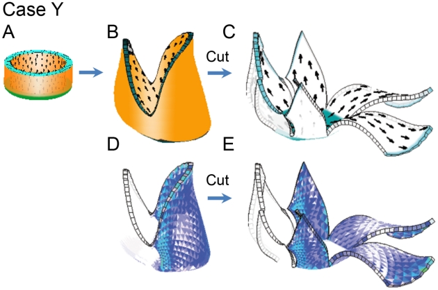
(A, B) Shape grown similarly to Figure 6 E. The specified growth rate is shown in orange. (D) As for (B) but showing the accumulated residual-strain (blue). Strain is not retained on the left side and is fully retained on the right side (strain retention is controlled through the action of which is only active on the right side). (C, E) The result of turning off growth, making 8 vertical cuts in the mature shape and allowing the shape to re-stabilise.

Figure 12. A curved canvas is approximated as a mesh of pentahedra.

Figure 13. Patterning in the canvas.

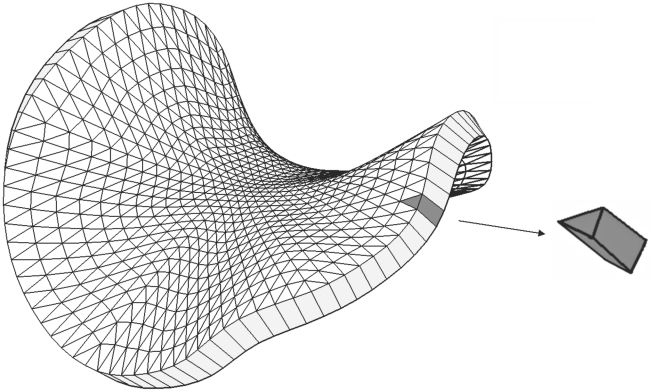
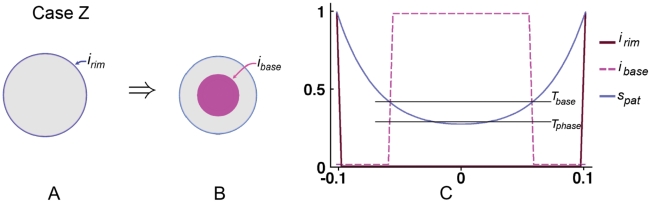
(A) The initial disc has a pre-defined region at the rim, (blue). (B) The inner region, (magenta), is obtained through a combination of diffusion and interaction of a signal () produced by . (C) Profiles of the factors (, , ) plotted along a diameter together with the thresholds, and .