Owl's behavior and neural representation predicted by Bayesian inference

Abstract

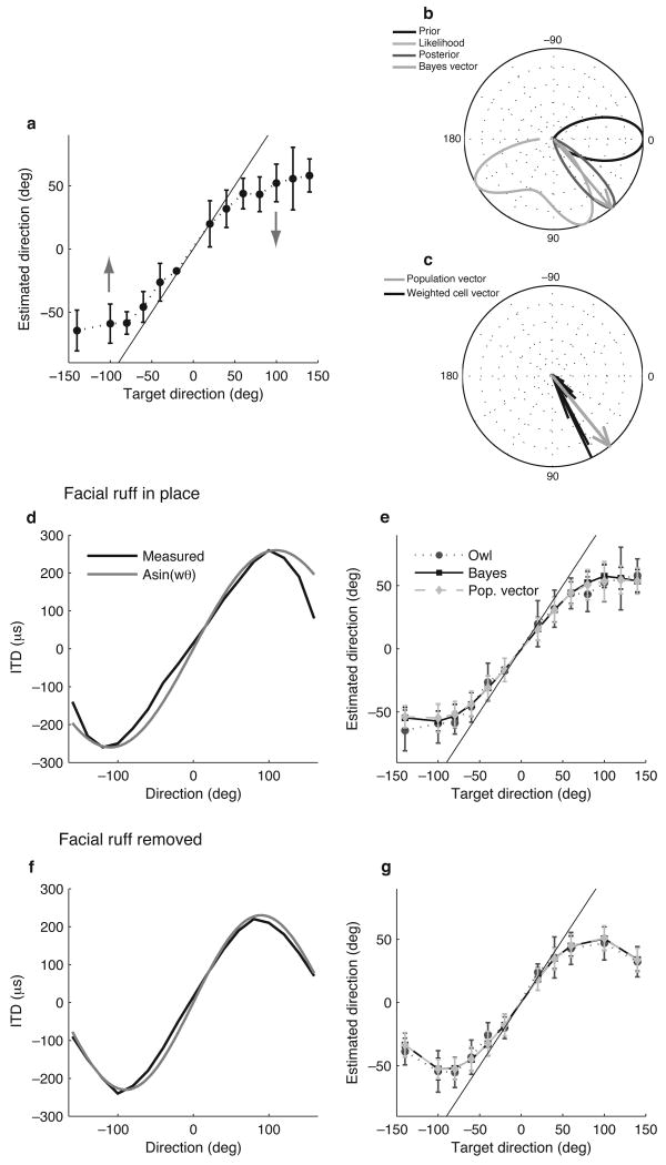
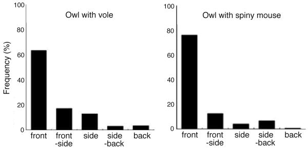
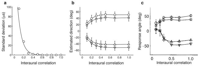
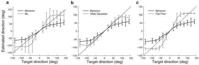
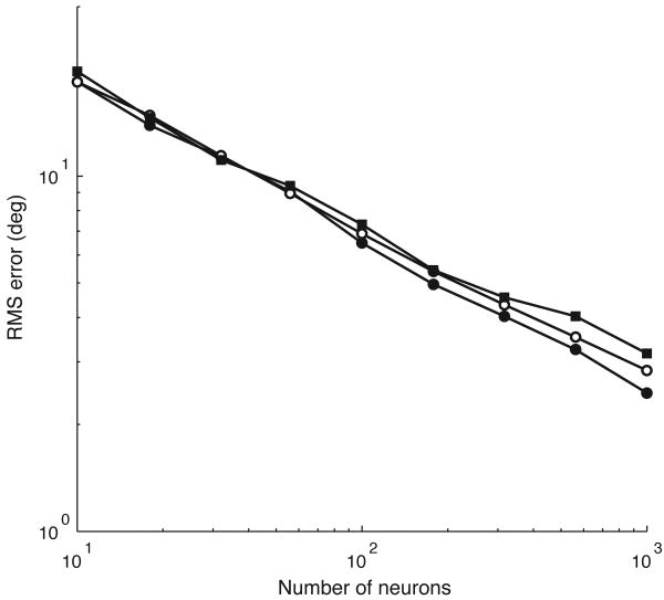
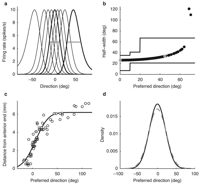
The owl captures prey using sound localization. In the classical model, the owl infers sound direction from the position of greatest activity in a brain map of auditory space. However, this model fails to describe the actual behavior. Although owls accurately localize sources near the center of gaze, they systematically underestimate peripheral source directions. We found that this behavior is predicted by statistical inference, formulated as a Bayesian model that emphasizes central directions. We propose that there is a bias in the neural coding of auditory space, which, at the expense of inducing errors in the periphery, achieves high behavioral accuracy at the ethologically relevant range. We found that the owl's map of auditory space decoded by a population vector is consistent with the behavioral model. Thus, a probabilistic model describes both how the map of auditory space supports behavior and why this representation is optimal.

Figure 1

Models of the owl's behavior. (a) Owl's behavior, modified from ref. 2. The solid gray line is the identity. (b) The Bayesian estimate is the direction of the vector found by averaging unit vectors in each direction weighted by the posterior density (medium gray). The posterior is proportional to the product of the likelihood (light gray) and the prior (black). All probablity densities were normalized by their peak for display. The source direction is 70 degrees, at one of the peaks of the likelihood. (c) The population vector (gray) is the average of the preferred direction vectors of the neurons, weighted by the firing rates (black). (d) Measured relationship between direction and interaural time difference (ITD) (black) under normal conditions, along with the sinusoidal approximation (gray). (e) Owl's behavior (medium gray circle, dotted line), Bayesian estimator (black square, solid line), and population vector (light gray diamond, dashed line) under the normal condition. Error bars represent the standard deviation over trials. (f) Measured relationship between direction and ITD (black) under ruff-removed conditions, along with the sinusoidal approximation (gray). (g) Owl's behavior, Bayesian estimator, and population vector under the ruff-removed condition.

Figure 2

Measured prior distribution of target direction. The relative frequency of different oppositions between an owl and two types of prey (vole on the left and spiny mouse on the right) during prey capture (modified from Fig. 3 in ref. 20). Front is the prey positioned at 0 deg relative to the owl's center of gaze, front-side corresponds to the regions centered at ± 45 deg, side corresponds to the regions centered at ± 90 deg, side-back corresponds to the regions centered at ± 135 deg, and back corresponds to the region centered at 180 deg.

Figure 3

Predicted behavior under varying levels of interaural correlation. (a) Variability of ITD with interaural correlation. ITD was estimated from the peak of the cross-correlation of the left and right input signals. (b) Direction estimates from the Bayesian model using levels of the standard deviation of the noise corrupting ITD that follow the exponential relationship shown in (a) with a minimum value of 41.2 μs, estimated from the behavioral data (s.d. = 219.34 exp(−11.31×IC)+41.2, where IC is the interaural correlation). Symbols correspond to four different source directions (± 55, ± 75 degrees). Error bars represent the standard deviation over trials. (c) The predicted trend is similar to observations in behaving owls (modified from Fig. 1 in ref. 21).

Figure 4

Performance of alternative estimators. (a) Owl's behavior (bold black) and maximum likelihood (ML) estimate (gray). The thin black line is the identity. Error bars represent the standard deviation over trials. (b) Owl's behavior (bold black) and Bayesian estimate using the mean of the posterior distribution when using a Gaussian-shaped prior that is wider than the optimal value (gray). (c) Owl's behavior (bold black) and Bayesian estimate using the mean of the posterior distribution when using a flat prior (gray).

Figure 5

Population vector approximation to Bayesian estimator. The root-mean-square (RMS) difference in direction estimates between the population vector and the Bayesian estimator for different correlation coefficients in the noise between neurons (black circles 0.25, white circles 0.5, black squares 0.75).

Figure 6

Predicted midbrain representation of auditory space. (a) Example tuning curves in the model optic tectum (OT) population. (b) Plot of model tuning curve half-widths (black circles) along with experimental data measured in the OT (solid lines, showing plus/minus 1 standard deviation, as reported in ref. 28). Gray and white circles correspond to the tuning curves highlighted in (a). The two outlier points correspond to receptive fields in the periphery that wrap around the owl's head, and which are indeed observed in the owl's OT data as well. (c) Measured values of space map positions of OT neurons (modified from ref. 28) together with the fit by a scaled cumulative Gaussian distribution function (solid line). (d) The model prior density of preferred direction (dashed gray) and the measured bilateral density (solid black) found by combining the unilateral densities derived from the cumulative Gaussian in (c).

References

1. Knudsen EI, Blasdel GG, Konishi M. Sound localization by the barn owl (Tyto alba) measured with the search coil technique. J Comp Physiol. 1979;133:1–11.
1. Hausmann L, von Campenhausen M, Endler F, Singheiser M, Wagner H. Improvements of sound localization abilities by the facial ruff of the barn owl (Tyto alba) as demonstrated by virtual ruff removal. PLoS ONE. 2009;4(11):e7721. doi: 10.1371/journal.pone.0007721. - DOI - PMC - PubMed
1. Populin LC, Yin TC. Behavioral studies of sound localization in the cat. J Neurosci. 1998;18:2147–2160. - PMC - PubMed
1. Jay MF, Sparks DL. Localization of auditory and visual targets for the initiation of saccadic eye movements. In: Berkley MA, Stebbins WC, editors. Comparative perception Basic mechanisms. Wiley, New York; New York, USA: 1990. pp. 351–374.
1. Nodal FR, Bajo VM, Parsons CH, Schnupp JW, King AJ. Sound localization behavior in ferrets: comparison of acoustic orientation and approach-to-target responses. Neuroscience. 2008;154:397–408. - PMC - PubMed
Publication types