A new way to see RNA

Abstract

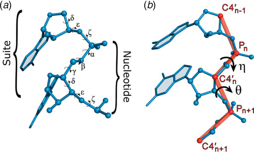
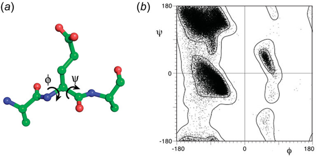
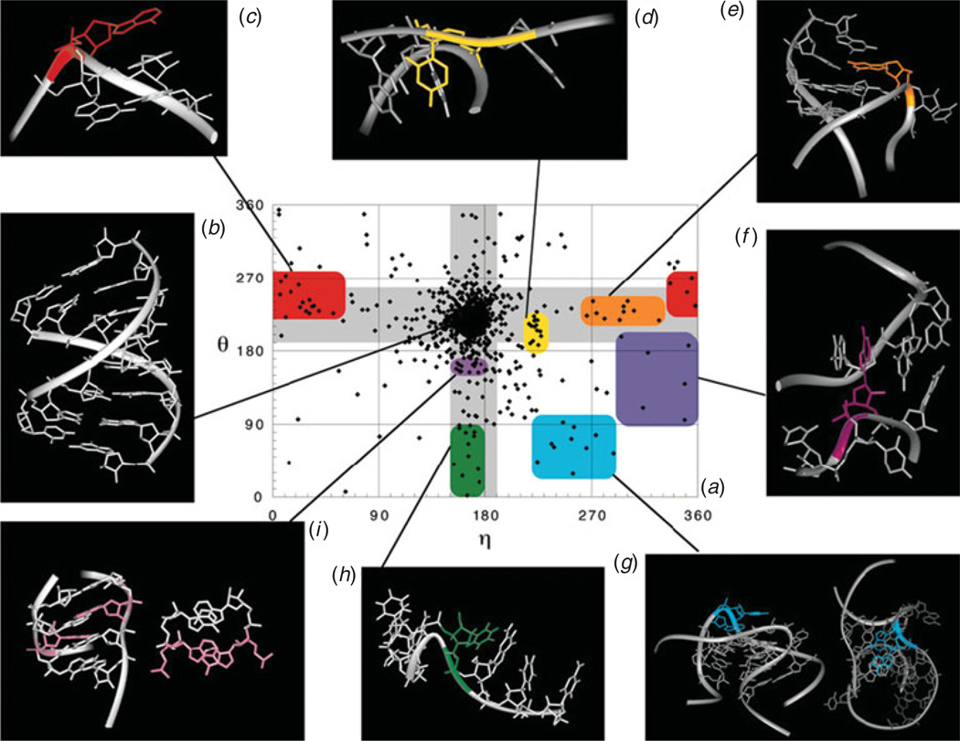
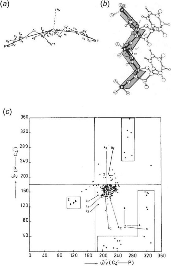
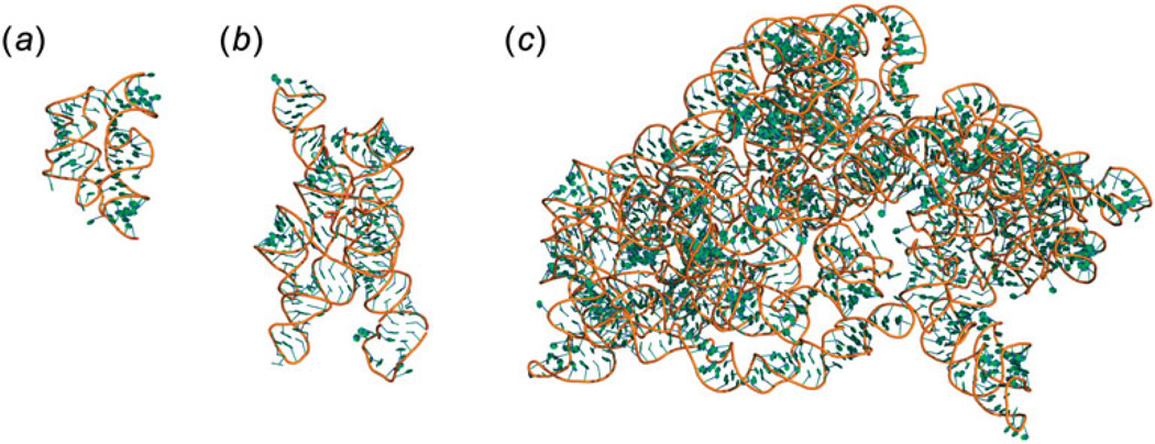
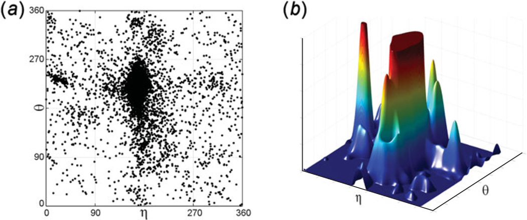
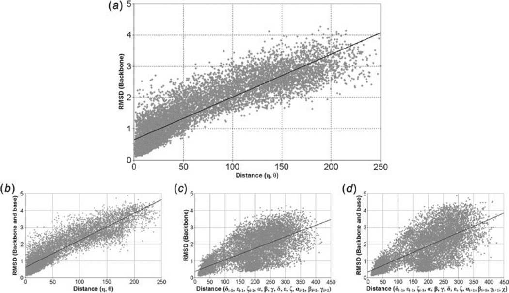
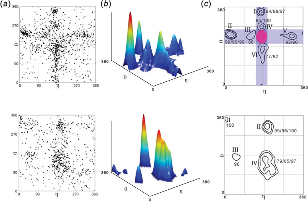
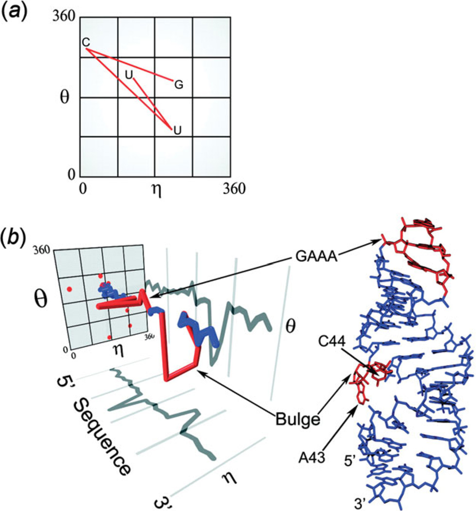
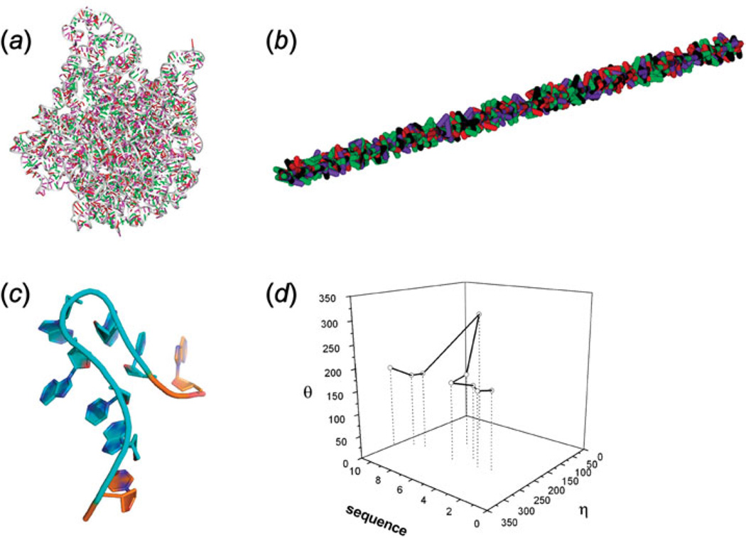
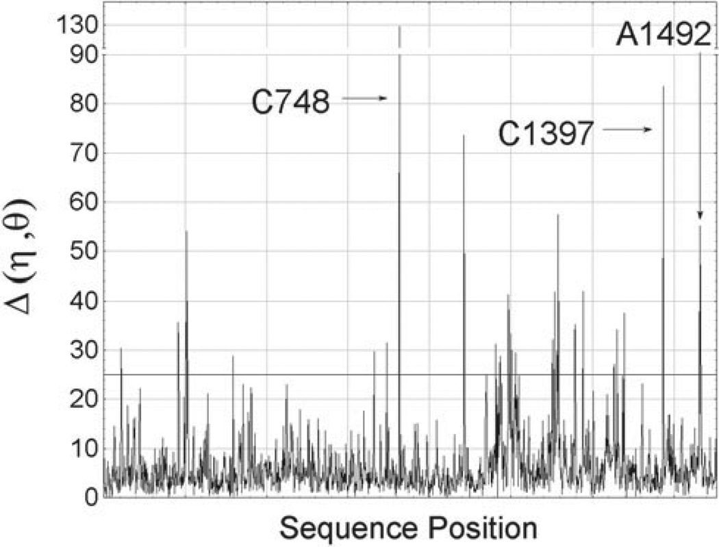
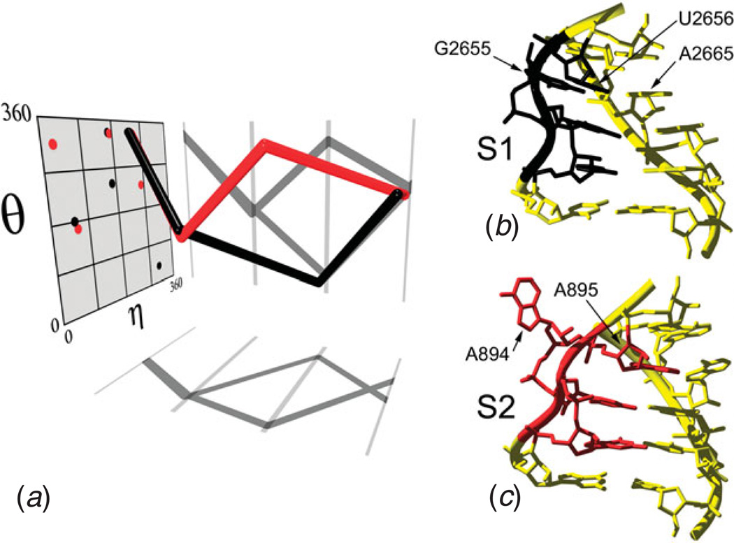
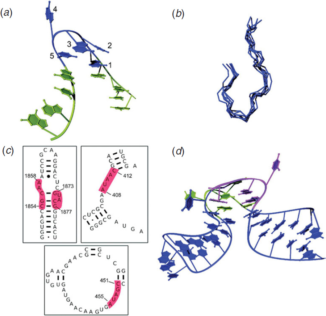
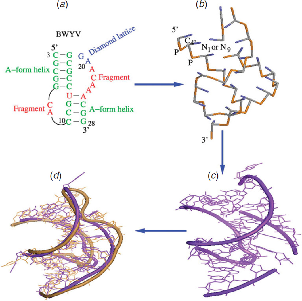
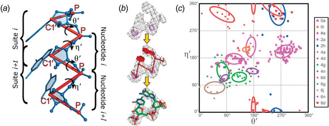
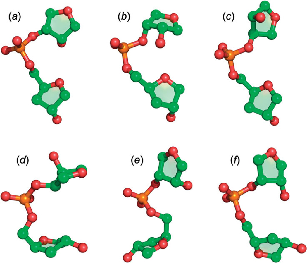
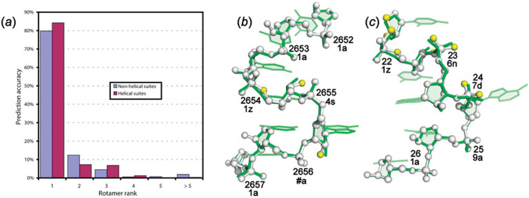
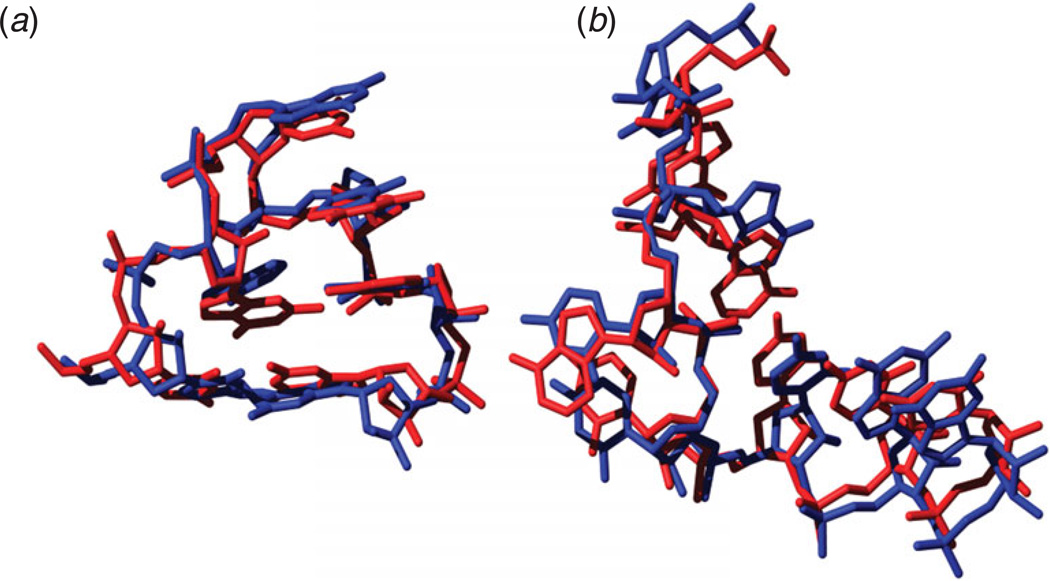
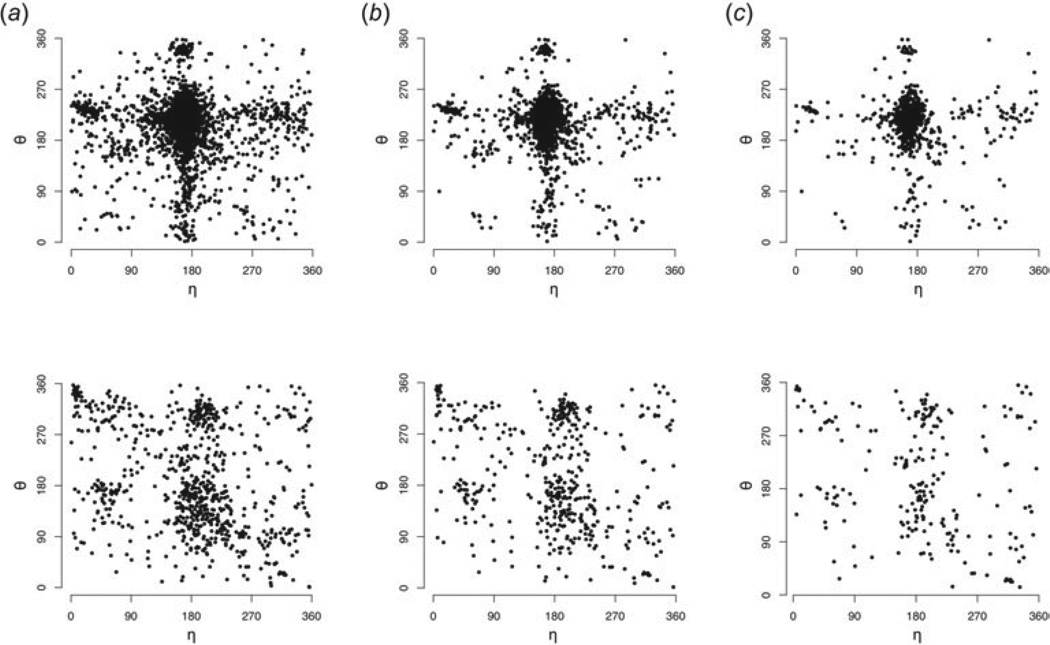
Unlike proteins, the RNA backbone has numerous degrees of freedom (eight, if one counts the sugar pucker), making RNA modeling, structure building and prediction a multidimensional problem of exceptionally high complexity. And yet RNA tertiary structures are not infinite in their structural morphology; rather, they are built from a limited set of discrete units. In order to reduce the dimensionality of the RNA backbone in a physically reasonable way, a shorthand notation was created that reduced the RNA backbone torsion angles to two (η and θ, analogous to φ and ψ in proteins). When these torsion angles are calculated for nucleotides in a crystallographic database and plotted against one another, one obtains a plot analogous to a Ramachandran plot (the η/θ plot), with highly populated and unpopulated regions. Nucleotides that occupy proximal positions on the plot have identical structures and are found in the same units of tertiary structure. In this review, we describe the statistical validation of the η/θ formalism and the exploration of features within the η/θ plot. We also describe the application of the η/θ formalism in RNA motif discovery, structural comparison, RNA structure building and tertiary structure prediction. More than a tool, however, the η/θ formalism has provided new insights into RNA structure itself, revealing its fundamental components and the factors underlying RNA architectural form.

Fig. 1

The RNA backbone. (a) Diagram of a nucleotide showing the six standard backbone torsion angles (α, β, γ, δ, ε, and ζ). The nucleotide and suite divisions of the backbone are indicated. A nucleotide is centered about the ribose sugar and spans two phosphates, while a suite is centered about the phosphate and spans two sugars. (b) Diagram depicting the definitions of the pseudo-torsions, η and θ. The red lines indicate the pseudo-bonds that connect successive P and C4′ atoms. The portion of the backbone shown affects a single pair of η and θ values, as the pseudo-torsions extend into the previous and next nucleotide. Figure modified from Wadley et al. (2007) with permission.

Fig. 2

The peptide backbone. (a) Diagram of a peptide showing the two variable backbone torsions (ϕ and ψ). (b) A Ramachandran plot of ϕ versus ψ showing approximately 81 000 non-glycine, non-proline and non-pre-proline residues from a high-resolution database, along with validation contours for favored and allowed regions. Figure reprinted from Lovell et al. (2003) with permission.

Fig. 3

Features of the η − θ plot, (a) An η − θ plot published in 1998 shows all nucleotides (from a database of 53 RNA structures. Gray bars represent areas of the plot where either η or θ is in the same range as nucleotides in the helical region. Colored areas are regions of the plot that contain nucleotides that share similar structural features. Note that η − θ plots from later analyses are shown in Figs 6, 8 and 20. (b)–(i) Representative nucleotides from the regions of the plot indicated. (b) The helical region: the intersection of the two gray bars include nucleotides from the crystal structure of an A-form duplex (from PDB file 1rxa; Portmann et al. 1995). (c) Stacked turn region; exemplified by the second nucleotide of a GNRA loop (PDB file 1zif, Ade 5; Jucker et al. 1996). id) The χ-switch region: includes the nucleotide 5′ to the cleavage site of the hammerhead ribozyme (PDB file 300d, Cyt B170; Scott et al. 1996). (e) Flip-turn region; exemplified by APK A27 G pseudo-knot nucleotide G9 (PDB file lkpd, Gua 9; Kang & Tinoco, 1997). (f) The C2′-bend region, includes tRNA^phe tertiary contact nucleotide G18 (PDB file 1tra, GUA 18; Westhof & Sundaralingam, 1986). (g) The stack switching region, exemplified by P456 domain pivot nucleotides (PDB file 1gid, nucleotides Ade A122, Ade A123; Cate et al. 1996). (b) The base twist region: includes the last stem nucleotide of a kissing hairpin (PDB file 1kis, Ura 21; Chang & Tinoco, 1997). (i) The cross-strand stack region: includes all 5′ nucleotides in sheared tandem R-R pairs (PDB file 1gid, Ade A113, Ade A206; Cate et al. 1996). Figure reprinted from Duarte & Pyle (1998) with permission.

Fig. 4

A phosphate- and C4′-based virtual bond system has been independendy developed three separate times. (a) The first such system was published in July of 1980 by Olson. Figure reprinted from Olson (1980) with permission. (b) Several months later – November, 1980 – Malathi and Yathindra independendy published an identical virtual bond system (Malathi & Yathindra, 1980). Figure reprinted from Malathi & Yathindra (1982) with permission. (c) An ω′_v − ω_v plot published in 1985 by Malathi and Yathindra (Malathi & Yathindra, 1985). The ω′_v angle is the torsion about the C4′-P virtual bond and is identical to θ, and the ω_v angle is the torsion about the P-C4′ virtual bond and is identical to η. (Note that the ω′_v and ω_v axes are reversed from those in the η − θ plots shown in Figs 3, 6, 8 and 20). The points on this plot represent nucleotides from oligonucleotide and yeast tRNA ^phe crystal structures. Figure reprinted from Malathi & Yathindra (1985) with permission.

Fig. 5

The late 1990s and early 2000s saw the publication of a wealth of complex RNA tertiary structures, including (a) the thiamine riboswitch (PDB ID: 1CKY; Thore etal. 2006), (b) the group I intron (PDB ID: 1U6B; Adams et al. 2004) and numerous ribosomal structures, (c) Shown here is the 16S ribosomal RNA from the bacterial 70S ribosome (PDB ID: 2JOO; Selmer et al. 2006). All structures are shown to scale. In each, the backbone is shown as an orange ribbon and the bases are shown in green.

Fig. 6

The effect of windowing an η − θ plot using a Blackman window function. (a) An η − θ scatter plot of all nucleotides from the (Wadley et al. 2007) dataset. Each point shows the η and θ values of an individual nucleotide. (b) The result of applying the Blackman window to the dataset, colored from low to high density: blue, green, yellow and red. An upper cut-off has been applied to allow for better discernment of the peaks surrounding the helical region. Figure modified from Wadley et al. (2007) with permission.

Fig. 7

Scatter plots of RMSD versus distance in the η–θ plane or standard torsional angles. For each plot, the best fit line for 10 000 random pairs of nucleotides from the dataset is shown. (a) RMSD of backbone atoms versus distance in the η–θ plane. The correlation coefficient is 0.80. (b) RMSD of backbone, sugar and base atoms versus distance in the η–θ plane. The correlation coefficient is 0.81. (c) RMSD of backbone atoms versus distance of standard torsional backbone angles. The correlation coefficient is 0.50. (d) RMSD of backbone, sugar and base atoms versus distance of the standard torsional angles (including χ). The correlation coefficient is 0.50. Figure reprinted from Wadley et al. (2007) with permission.

Fig. 8

Clusters of non-helical nucleotides in the η − θ plot become more apparent after the dataset is divided by sugar pucker. (a) A scatter plot of the η − θ values of all non-helical C3′-endo (top) and C2′-endo (bottom) nucleotides. (b) A 3D view of the plot of C3′-endo (top) and C2′-endo (bottom) nucleotides with a 60° wide Blackman window function applied. (c) A contour plots resulting from analyzing the C3′-endo (top) and C2′-endo (bottom) density plots in (b). Contour levels are shown at 1σ, 2σ and 4σ levels, and scores are given in that order. These cluster scores report the percentage of nucleotides within the specified region that are superimposable with the corresponding prototype nucleotide. Contours with small populations (< 9) are not shown. The blue bars span the helical η values and the helical θ values for C3′-endo nucleotides. The pink elliptical area near the center of plot indicates the helical region that was initially excluded from the analysis. Figure modified and reprinted with permission from Wadley et al. (2007).

Fig. 9

RNA motifs can be identified using η − θ worms. (a) A two-dimensional representation of the worm for the UUCG tetraloop motif. (b) A three-dimensional representation of a worm for the group II intron domain V structure (Sigel et al. 2004). This worm clearly reveals the location of a GAAA tetraloop and an extra-helical bulge (both of which are indicated in red on the worm and the structure). Figure reprinted from Duarte et al. (2003) with permission.

Fig. 10

PRIMOS analysis of the ribosome. (a) The tertiary structure of the 50S subunit of the ribosome (Ban et al. 2000). (b) The 50S subunit represented as an η − θ worm. (c) The hook turn, a motif found in the ribosome that was initially identified using PRIMOS (Szep et al. 2003). (d) A three-dimensional worm for the hook-turn motif. (d) Reprinted from Szep et al. (2003) with permission.

Fig. 11

PRIMOS analysis can reveal changes between two related structures. Here, two 30S structures are compared: one unbound (PDB code IBL; Ogle et al. 2001) and one bound by paromomycin and a tRNA anticodon stem-loop (PDB code 1KQS; Schmeing et al. 2002). The line at 25° indicates a threshold above which nucleotides are considered to have different conformations in each complex. Some regions undergoing conformational changes between the complexes are indicated: the A site (A1492), the P site (C1397) and a site in the platform domain (C748). Figure reprinted from Duarte et al. (2003) with permission.

Fig. 12

Pseudo-torsion analysis using PRIMOS revealed that there are two types of S-turn motifs, referred to as the SI (classical S-turn) motif and the S2 motif. (a) Characteristic RNA worms for analogous portions of S1 (black) and S2 (red) motifs. (b) S1-motif structure with backbone ribbon (PDB code: 480D; Chang & Tinoco, 1997). Nucleotides for the S1 worm (U2653-U2656) are in black. (c) S2-motif structure (PDB code: 1JJ2; Klein et al. 2001). Nucleotides for the S2 worm (G892-A895) are in red. Figure reprinted from Duarte et al. (2003) with permission.

Fig. 13

The COMPADRES technique was used to identify a number of novel motifs, including the π-tutn shown here. (a) An example of an isolated π-turn (PDB file, 1JJ2 0 :A408-C12; Klein et al. 2001) (from the 50S ribosomal subunit of Haharcula marismortui (H50S). The five structurally similar nucleotides (blue) are flanked by two helical strands (yellow). Numbering is from 5′ to 3′. (b) A superposition of the backbones of the seven π-turns found in our dataset. (c) Locations of the four H50S π-turns (highlighted in red) in secondary structure. (d) Two of the π-turns found in the H50S occurred symmetrically opposite each other, shown here in their helical context. Nucleotides not part of the canonical π-turns are shown in blue. Figure reprinted from Wadley & Pyle (2004) with permission.

Fig. 14

The VFold model, which is based on the η and θ pseudo-torsions, can be used to predict RNA tertiary structure and folding (Cao et al. 2010). Here, it is used to predict the three-dimensional structure of a pseudo-knot. (a) The predicted pseudo-knot secondary structure. (b) The predicted virtual-bond level tertiary structure. (c) The all-atom structure constructed from the scaffold shown in (b). (d) The all-atom structure after additional refinement. Figure reprinted from Cao et al. (2010) with permission.

Fig. 15

Typical RNA electron density maps for structures solved at various resolutions. Structures shown in (b–i) were retrieved from the Nucleic Acid Database (Berman et al. 1992), and electron density maps were calculated using observed structure factors and calculated phases, (a) Pie chart showing the resolutions of all large RNA structures (structures that contain a chain of at least 25 nucleotides), as retrieved from the Nucleic Acid Database (Berman et al. 1992). Numbers in parentheses are the number of structures in the specified resolution range. Note that structures in the 2.5–3.5-Å resolution range account for nearly two-thirds of all large RNA structures, whereas protein structures are typically solved at far higher resolutions. Maps are shown at (b) 1.04, (c) 1.75, (d) 2.25, (e) 2.75, (f) 3.3, (g) 3.8, (h) 4.5 and (i) 6.21 Å resolutions. Figure reprinted from Keating & Pyle (2010) with permission.

Fig. 16

RCrane uses the pseudo-torsions for crystallographic model building. (a) The η and θ′ pseudo-torsions, which use the C1′ atom in place of C4′. Additionally, the suite and nucleotide divisions of the backbone are indicated. (b) The model building process. Starting with the experimental electron density (top), a crystallographer builds phosphates and bases (middle). The detailed backbone structure can then be automatically predicted and constructed (bottom). (c) A θ′ − η′ plot showing suites of the RNA05 filtered dataset (Richardson et al. 2008). Each color and shape combination corresponds to a specific conformer as indicated in the key. Ellipses correspond to the Gaussian functions (at the 1σ level) used in conformer predictions. Only conformers with leading C2′ endo sugar pucker and ending C3′ endo sugar pucker are shown. Figure reprinted from Keating & Pyle (2010) with permission.

Fig. 17

The consensus backbone conformers describe 46 allowable configurations for the RNA backbone (Richardson et al. 2008). Here, sample backbone structures of six of these conformers are shown. Note that the consensus conformers use the suite division of the backbone rather than the nucleotide division (See Figs. 1a and 16a).

Fig. 18

The RCrane method results in highly accurate backbone structure. (a) Jackknife validation shows that conformer predictions are highly accurate. Prediction accuracy for conformers ranked as most likely, second most likely, etc., by the conformer prediction process. Standard error is <0.3% for all bars. (b, c) The sarcin/ricin domain (PDB code: 1Q9A; Correll et al. 2003) and guanine riboswitch (PDB code: 2EES; Gilbert et al. 2007) crystal structures were rebuilt using RCrane. The rebuilding used only the published phosphate and base coordinates, and was able to accurately and automatically reconstruct the backbone. Shown here are (b) the S-motif from the sarcin/ricin domain and (c) the J1/2 linker from the guanine riboswitch. The original structures are shown as green sticks and the rebuilt structures are shown in ball-and-stick representation. Atoms built within 0.5 Å of the published coordinates are shown as white spheres, and atoms built within 0.8 Å are shown in yellow. Suite numbers and conformers are labeled. Note that the rebuilt structure has not been minimized or refined against the electron density. Figure reprinted from Keating & Pyle (2010) with permission.

Fig. 19

RNA strands can be accurately rebuilt by computationally joining nucleotides with similar η/θ values from other structures. (a) An example of an in silico tetraloop superimposed on the original (1S72 0:8994; Klein et al. 2004). The backbone RMSD of the in silico strand (red) to the original tetraloop (blue) is 0.78 Å, despite the fact the nucleotides used to build the strand do not belong to any naturally occurring tetraloop. (b) A bulge region (1S72 0:1391–1398; Klein et al. 2004) from the 50 S ribosomal subunit. The in silico strand (blue) superimposed on the original (red) with a backbone RMSD of 0.91 Å. Figure reprinted from Wadley et al. (2007) with permission.

Fig. 20

Data filtering is important for η − θ plots. All plots shown here were constructed using the RNA05 dataset (Richardson et al. 2008) with differing filtering criteria. (a) Plots with no filtering applied. 7,372 C3′-endo (top) and 791 C2′-endo (bottom) nucleotides are shown, (b) Plots where nucleotides containing atoms with B factors >60 have been excluded. 3733 C3′-endo (top) and 458 C2′-endo (bottom) nucleotides remain. (c) Plots with additional quality filters applied to remove nucleotides containing a steric clash (van der Waals overlap > 0.4 Å, as measured by MolProbity clashscore; Word et al. 1999). 1548 nucleotides C3′-endo (top) and 218 C2′-endo (bottom) nucleotides remain and are shown in the plot. Note that for all plots in a–c, only nucleotides with a well-defined sugar pucker are shown (C3′-endo: δ = 84 ± 30, pseudo-phase angle of furanose ring (Saenger, 1984) between 0°–36° ± 18°, base–phosphate perpendicular distance >2.9 Å; C2′-endo: (δ = 147 ± 30, pseudo-phase angle of furanose ring between 144°–180° ± 18°, base-phosphate perpendicular distance ≤2.9 Å). Additionally, for nucleotides with alternative conformations, only the first instance listed in the pdb file was used.

References

1. Abramovitz DL, Friedman RA, Pyle AM. Catalytic role of 2′-hydroxyl groups within a group II intron active site. Science. 1996;271:1410–1413. - PubMed
1. Adams PL, Stahley MR, Kosek AB, Wang J, Strobel SA. Crystal structure of a self-splicing group I intron with both exons. Nature. 2004;430:45–50. - PubMed
1. Ban N, Nissen P, Hansen J, Moore PB, Steitz TA. The complete atomic structure of the large ribosomal subunit at 2.4 Å resolution. Science. 2000;289:905–920. - PubMed
1. Batey RT, Gilbert SD, Montange RK. Structure of a natural guanine-responsive riboswitch complexecd with the metabolite hypoxanthine. Nature. 2004;432:411–15. - PubMed
1. Beckers ML, Melssen WJ, Buydens LM. Predicting nucleic acid torsion angle values using artificial neural networks. Journal of Computer-Aided Molecular Design. 1998;12:53–61. - PubMed
Publication types