Two-dimensional adaptation in the auditory forebrain

Abstract

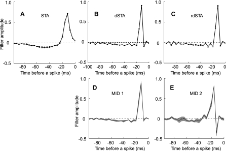
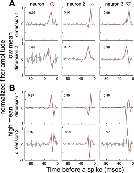
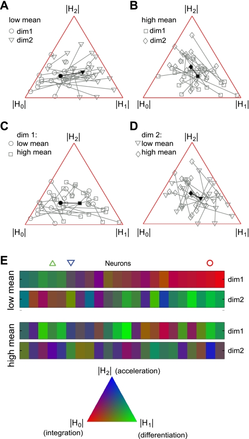
Sensory neurons exhibit two universal properties: sensitivity to multiple stimulus dimensions, and adaptation to stimulus statistics. How adaptation affects encoding along primary dimensions is well characterized for most sensory pathways, but if and how it affects secondary dimensions is less clear. We studied these effects for neurons in the avian equivalent of primary auditory cortex, responding to temporally modulated sounds. We showed that the firing rate of single neurons in field L was affected by at least two components of the time-varying sound log-amplitude. When overall sound amplitude was low, neural responses were based on nonlinear combinations of the mean log-amplitude and its rate of change (first time differential). At high mean sound amplitude, the two relevant stimulus features became the first and second time derivatives of the sound log-amplitude. Thus a strikingly systematic relationship between dimensions was conserved across changes in stimulus intensity, whereby one of the relevant dimensions approximated the time differential of the other dimension. In contrast to stimulus mean, increases in stimulus variance did not change relevant dimensions, but selectively increased the contribution of the second dimension to neural firing, illustrating a new adaptive behavior enabled by multidimensional encoding. Finally, we demonstrated theoretically that inclusion of time differentials as additional stimulus features, as seen so prominently in the single-neuron responses studied here, is a useful strategy for encoding naturalistic stimuli, because it can lower the necessary sampling rate while maintaining the robustness of stimulus reconstruction to correlated noise.

Fig. 1.

Firing rate predictions using one-dimensional (1D) and two-dimensional (2D) linear/nonlinear models. A: a segment of the randomly varying modulation signal σ that specifies the local log-amplitude of the sound in decibels (see materials and methods). B: responses of a single unit to 32 repetitions of the modulation signal shown in A. In one-half of all trials for each neuron, such repeated stimuli were presented (to use for predictions, as in C), while in the other one-half of trials, unrepeated versions of the modulation signal were presented and used to calculate the relevant dimensions and nonlinear gain functions of the linear-nonlinear (LN) models. C: real (black) and predicted firing rates for this example neuron using the 2D (pink) or 1D (blue) LN model. Neuron “eb1940”.

Fig. 2.

Comparison of different methods for characterizing neural feature selectivity. A: the dimension obtained as the so-called spike-triggered average (STA). B: decorrelated STA (dSTA). C: regularized decorrelated STA (rdSTA). The first (D) and second (E) most informative dimensions (MID) (see text for method description) are shown. In D and E, the MID results are plotted for optimizations starting with the STA (black line), and starting with a random stimulus segment (gray lines denote mean 1 SD). The two cases are almost indistinguishable, which proves that the algorithm is not sensitive to initial conditions. Neuron “soba1980”.

Fig. 3.

A population analysis of predictive power based on 2D linear/nonlinear models. A: the percentage of total information between spikes and stimulus accounted for by the 2D model vs. the percentage accounted for by the 1D model based on the first MID alone. Inset shows a histogram of the number of spike-triggered covariance method dimensions for each cell in our data set. The distribution peaks at two dimensions for all stimulus conditions. B: the percentage of variance in the firing rate accounted for by the 2D model vs. the percentage accounted for by the 1D model based on the first MID alone. The percentages for information and variance were computed using a novel segment of the data. Error bars are standard errors.

Fig. 4.

Shapes of the primary and secondary stimulus dimensions are strongly affected by mean sound volume. A: the primary and secondary stimulus dimensions for three example neurons are shown when the mean sound volume was low. The x-axis represents the time before a spike (at zero), and the y-axis represents normalized amplitude of the filter. B: results for the same neurons when the mean sound amplitude was high. Dark lines show the mean and standard deviation of dimensions as derived from data. Light gray lines show first time derivatives of the other dimension under each stimulus condition. Derivative comparisons are provided for the dimensions that were better approximated by the time derivative of the other dimension in the pair. From left to right, columns neuron IDs are “ra2200”, “soba1740wide”, and “udon2120”. See also Fig. 5 for fits using Hermite functions.

Fig. 5.

The relevant dimensions at low and high sound volume fitted with Hermite functions. Notations and neurons are the same as in Fig. 4. Red lines indicate fits using the three lowest order Hermite functions. Numbers within each panel show correlation coefficients between the relevant dimensions and their fits.

Fig. 6.

A population analysis of the shapes of relevant dimensions. The triplet of Hermite coefficients is represented as a dot within an equilateral triangle. A–D: comparison of pairs of dimensions under either the same or different stimulus conditions. Data from each cell are linked, and the dark vector shows the population mean. A: comparison of two relevant dimensions under the low mean stimulus condition. B: same as A, but for the high mean stimulus condition. C: comparison of primary dimensions between the low and high mean stimulus conditions. D: same as C, but for the secondary dimensions. E: by using color to represent the location within the reference triangle (bottom), we could compare the primary and secondary dimensions for each neuron within and across stimulus conditions (each neuron is represented in a vertical column). Red-green colors, corresponding to integration-differentiation, dominate in the low mean stimulus condition, whereas blue-green colors (differentiation-acceleration) dominate in the high mean stimulus condition. Symbols (circle, upward and downward triangles) label points corresponding to the example neurons from Fig. 4.

Fig. 7.

The time course of adaptation. A: the mean population response to the same (repeated) stimulus segment in the low mean/low variance condition is different, depending on the previous state of adaptation. Neurons were previously adapted to either the high mean/low variance condition (black line) or the low mean/high variance condition (gray line). The effect of the previous adaptation condition disappeared after 100 ms. Inset at top right shows the stimulus as it transitions from two different stimulus statistics conditions to the low mean/low variance stimulus condition (transition is marked by tick marks). B: the mean firing rate across the population of cells recorded, after a switch from low to high mean stimulus. The mean firing rate at each moment in time was estimated for each cell from a large number of different (unrepeated) noise segments and then averaged across cells. Thus stimuli are the same, on average, at each point in time. The decrease in mean firing rate reflects the difference in average neural responses to the same average stimuli, indicating an adaptive process. The solid black line shows an exponential fit to the data (black), and the corresponding time constant is provided in the inset. P value corresponds to an F-test comparing an exponential fit with the null hypothesis of no time dependence. Error bars show standard errors of the mean. C: the first MID estimated in the stationary state provides an increasingly better description of neural responses with time following a switch to high mean stimulus condition. Each data point represents the average amount of information explained across the population of neurons to the same stimulus segment. Black line and inset are as in B. The larger variability in C compared with B stems from the fact that it is based on the population neural response to a single stimulus segment (repeated responses to the same stimulus are required for the information calculation), whereas, in B, averaging was done with respect to different stimulus segments and thus much more data.

Fig. 8.

Effects of stimulus variance on the 2D nonlinear gain functions for two example neurons (A/B and C/D). Gray-scale plots show the firing rate in Hz as a function of the two relevant stimulus components. Thin black lines show regions where values are >2 SE. The average firing rate as a function of individual components of the stimulus is shown in side plots (gray and black lines for the high- and low-variance conditions, respectively; the gray lines of the high variance condition are replotted in the right half of the figure for comparison). Stimulus components are normalized to have unit variance and plotted in units of standard deviation. Top row is one neuron (“udon2120”); bottom row is a different neuron (“eb1940”). Although the gain of 2D functions shows some rescaling with stimulus variance (compare columns), it is not complete for secondary dimensions, and in some cases (e.g., bottom row) the shape of the secondary filters can change qualitatively.

Fig. 9.

Contribution of secondary dimensions to neural firing increases with stimulus variance. We measure relative information gain by computing a difference between the information accounted for by two dimensions (Info_2D) and that accounted for by the primary dimension alone (Info_1D), and then dividing by Info_2D. Such a ratio represents a way to measure the relative influence of the two dimensions on neural firing. A ratio different from one indicates a change in the shape of the nonlinear gain function relative to the stimulus probability distribution, for example, due to imperfect or uneven rescaling of firing rate gain with respect to relevant stimulus dimensions. Shown are the low mean/low variance stimulus condition (x-axis) vs. low mean/high variance condition (y-axis). Across the population of neurons, the contribution of the second dimension was significantly larger in the high variance compared with the low-variance condition (P = 0.0156, paired Wilcoxon test). Points that lie significantly above the line indicate that the inclusion of a second dimension increased the information more in the high variance condition than in the low; points below the line indicate more information from a second dimension in the low-variance condition. Each symbol is a neuron, black P < 0.05, white P > 0.05, t-test. Neurons exhibiting a significant change in the shape of the 2D gain function were characterized by a weaker contribution of the second dimension with a low-variance stimulus (7/8). The points marked with symbols are the same as in Fig. 8.

Fig. 10.

The distribution of spike-time jitter. A: spike-time jitter was estimated following the method of Aldworth et al. (2005), whereby estimates of the relevant stimulus dimension (computed as STA) are readjusted by allowing varying delays in the arrival times of single spikes. The standard deviation of a Gaussian distribution for jitter in spike time was computed separately for each cell and stimulus condition. The three outlier points belong to the same neuron “pho1295wide” under the three different stimulus conditions. Thus nearly all cells exhibit a very low degree of spike-time jitter with submillisecond precision in spike timing. In B and C, we illustrate typical results of MID optimization obtained with (thick gray line) and without prior dejittering of spike trains binned at 4-ms resolution. The subspace projection between the two relevant spaces for this example is 0.99. Neuron “udon2120”.

Fig. 11.

Different sampling strategies and their susceptibility to noise. A: in traditional sampling, function values are measured at an average rate of 2W, where W is the signal bandwidth. B: when the signal and its time differential are sampled simultaneously, measurements can be done at the reduced rate of W. C: when the signal and its first and second time differentials are measured together, the sampling rate can be further reduced to 2W/3. All three strategies are equivalent in the absence of noise. D: illustration of the effects of noise on the computation of derivatives. Top: signal with no noise. Middle: in the presence of high-frequency noise, nearby time points have very different noise values, making the computation of time-derivatives noisy (Wτ = 0.1). Bottom: in the presence of low-frequency noise, nearby time points generally have similar noise values, making the derivative computation more robust (Wτ = 1.0). E: mean reconstruction error in a linear model where sample values are corrupted by noise. The results are plotted as a function of noise correlation time τ. Blue line, traditional sampling of signal values; left magenta line, sampling of signal and first time derivatives; right brown line, sampling of signal, first and second time derivatives.

References

1. Abramowitz M, Stegun IA. Handbook of Mathematical Functions. Washington, DC: US Government Printing Office, 1964
1. Adelman TL, Bialek W, Olberg RM. The information content of receptive fields. Neuron 40: 823–833, 2003 - PubMed
1. Agüera y Arcas B, Fairhall AL. What causes a neuron to spike? Neural Comput 15: 1789–1807, 2003 - PubMed
1. Agüera y Arcas B, Fairhall AL, Bialek W. Computation in a single neuron: Hodgkin and Huxley revisited. Neural Comput 15: 1715–1749, 2003 - PubMed
1. Aldworth ZN, Miller JP, Gedeon T, Cummins GI, Dimitrov AG. Dejittered spike-conditioned stimulus waveforms yield improved estimates of neuronal feature selectivity and spike-timing precision of sensory interneurons. J Neurosci 25: 5323–5332, 2005 - PMC - PubMed
Publication types
LinkOut - more resources