Quantification and compensation of eddy-current-induced magnetic-field gradients

Abstract

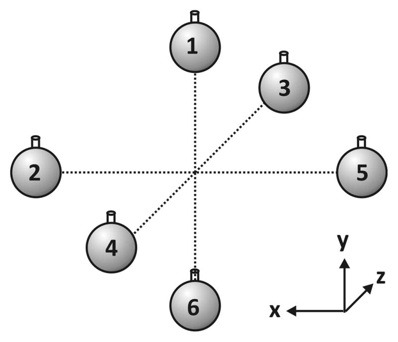
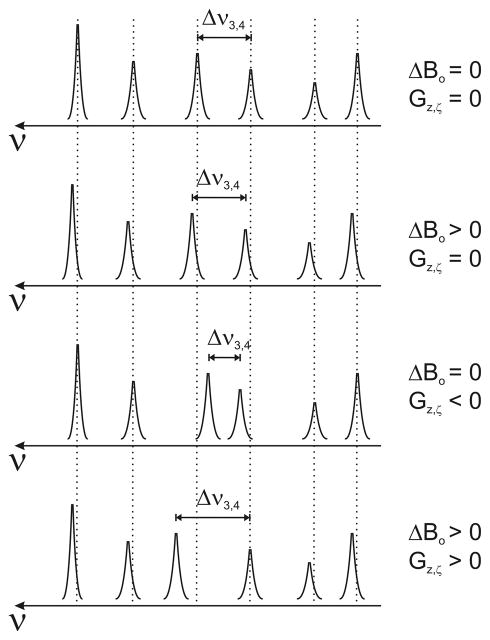
Two robust techniques for quantification and compensation of eddy-current-induced magnetic-field gradients and static magnetic-field shifts (ΔB0) in MRI systems are described. Purpose-built 1-D or six-point phantoms are employed. Both procedures involve measuring the effects of a prior magnetic-field-gradient test pulse on the phantom's free induction decay (FID). Phantom-specific analysis of the resulting FID data produces estimates of the time-dependent, eddy-current-induced magnetic field gradient(s) and ΔB0 shift. Using Bayesian methods, the time dependencies of the eddy-current-induced decays are modeled as sums of exponentially decaying components, each defined by an amplitude and time constant. These amplitudes and time constants are employed to adjust the scanner's gradient pre-emphasis unit and eliminate undesirable eddy-current effects. Measurement with the six-point sample phantom allows for simultaneous, direct estimation of both on-axis and cross-term eddy-current-induced gradients. The two methods are demonstrated and validated on several MRI systems with actively-shielded gradient coil sets.

Figure 1

Geometry of the Six-Point-Sample (3-D) Phantom. The time-dependent frequency shift between a pair of point solvents aligned along a given principal axis is used to monitor the time-dependent, eddy-current-induced gradients in that direction.

Figure 2

Schematic representation of the spectral response from the six-point (3-D) phantom in the presence of eddy-current-induced gradients and ΔB_o-field shifts.

Figure 3

Prior to eddy-current compensation, a general trend toward higher eddy-current-induced gradients with greater d_grad/d_magnet is observed for the sample of MRI systems in this study. The quantity d_grad represents the gradient i.d., while d_magnet is the magnet bore diameter. For purposes of this plot, overall eddy-currents are represented as a sum of all of the on-axis (x → x, y → y, z → z) eddy-current decay components shown in Table 3 (e.g., in terms of Eq. 15, Σ_{j = x,y,z} Σ_i A_i ×100%).

Figure 4

Measured diagonal, z → z, eddy-current-induced gradients ([G_z,ζ/G_z,test] × 100%) in MRI system #1 (see Table 2 for system specifications) vs. delay time, δ, between the falling edge of the gradient test-pulse and the start of the FID acquisition. For the six-point sample (3-D) measurement (□), the gradient parameters were 2.5 s duration, 1 G/cm gradient amplitude; for the 1-D sample measurement (●), the gradient parameters were 2.5 s duration, 6 G/cm gradient pulse. After compensation, negligible eddy-current gradients remained as evidenced by results from the six-point sample measurement (■) and 1-D sample measurement (○) after properly setting the gradient pre-emphasis.

Figure 5

Single-shot EPI images of a sample of PEG 400 (polyethylene glycol, mol. wt._ave = 400 g/mol) contained within a 5 cc syringe. In addition to the PEG 400 liquid, the lumen of the syringe contains the ×-shaped piston taken from another identical 5 cc syringe. Both images were acquired at 4.7 T with system #2 (after proper eddy-current compensation) from a 2-mm thick slice with a 14 × 14 mm² (64 × 64) field-of-view using a spin-echo preparation (TE = 97 ms). Left. Image acquired without diffusion weighting (b = 0). Right. Heavily diffusion-weighted (b = 534,000 s/mm²) image of the sample employing a pair of trapezoidal gradient pulses on either side of the spin-echo refocusing pulse (G = 40 G/cm, δ = 25 ms, Δ = 33.2 ms, applied simultaneously along all three Cartesian axes).

References

-
- Jehenson P, Syrota A. Correction of Distortions due to the Pulsed Magnetic Field Gradient-Induced Shift in Bo Field by Postprocessing. Magnetic Resonance in Medicine. 1989;12:253–256. - PubMed
- Terpstra M, Andersen PM, Gruetter R. Localized eddy current compensation using quantitative field mapping. Journal of Magnetic Resonance. 1998;131:139–143. - PubMed
- de Graaf RA. In Vivo NMR Spectroscopy. John Wiley & Sons; Chichester, U.K: 2007.
- Gibbs SJ, Johnson CS. A PFG NMR Experiment for Accurate Diffusion and Flow Studies in the Presence of Eddy Currents. Journal of Magnetic Resonance. 1991;93:395–402.
- Jezzard P, Barnett AS, Pierpaoli C. Characterization of and Correction for Eddy Current Artifacts in Echo Planar Diffusion Imaging. Magnetic Resonance in Medicine. 1998;39:801–812. - PubMed
Publication types
MeSH terms
Substances
Grants and funding
LinkOut - more resources
Full Text Sources
Other Literature Sources