Components of cross-frequency modulation in health and disease

Abstract

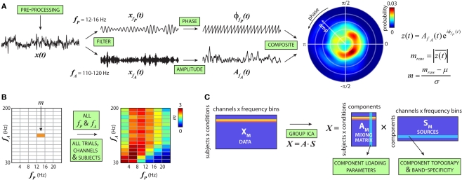
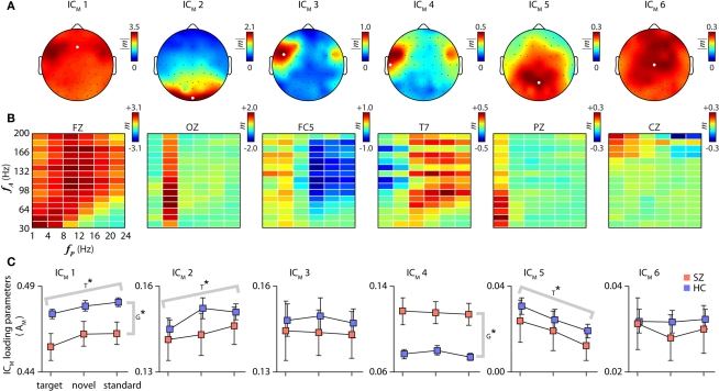
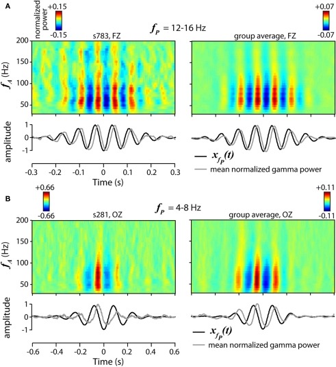
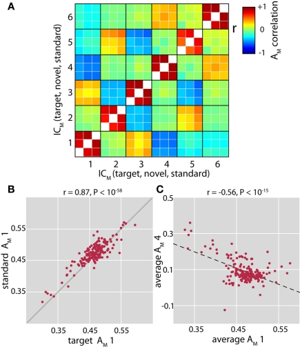
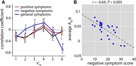
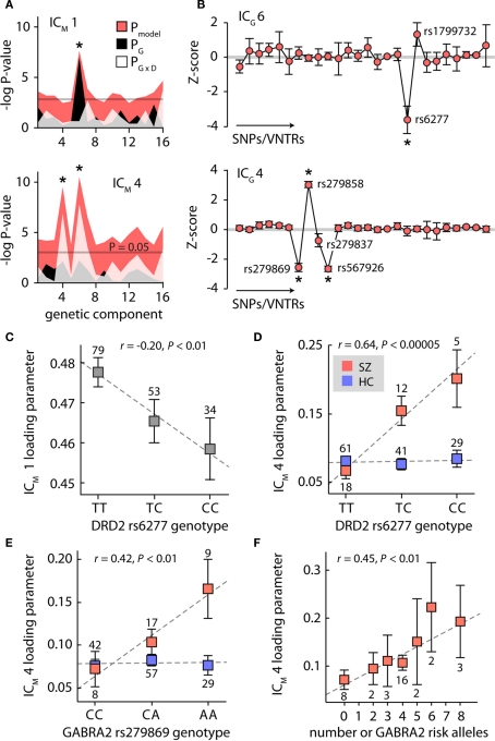
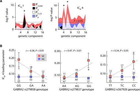
The cognitive deficits associated with schizophrenia are commonly believed to arise from the abnormal temporal integration of information, however a quantitative approach to assess network coordination is lacking. Here, we propose to use cross-frequency modulation (cfM), the dependence of local high-frequency activity on the phase of widespread low-frequency oscillations, as an indicator of network coordination and functional integration. In an exploratory analysis based on pre-existing data, we measured cfM from multi-channel EEG recordings acquired while schizophrenia patients (n = 47) and healthy controls (n = 130) performed an auditory oddball task. Novel application of independent component analysis (ICA) to modulation data delineated components with specific spatial and spectral profiles, the weights of which showed covariation with diagnosis. Global cfM was significantly greater in healthy controls (F(1,175) = 9.25, P < 0.005), while modulation at fronto-temporal electrodes was greater in patients (F(1,175) = 17.5, P < 0.0001). We further found that the weights of schizophrenia-relevant components were associated with genetic polymorphisms at previously identified risk loci. Global cfM decreased with copies of 957C allele in the gene for the dopamine D2 receptor (r = -0.20, P < 0.01) across all subjects. Additionally, greater "aberrant" fronto-temporal modulation in schizophrenia patients was correlated with several polymorphisms in the gene for the α2-subunit of the GABA(A) receptor (GABRA2) as well as the total number of risk alleles in GABRA2 (r = 0.45, P < 0.01). Overall, our results indicate great promise for this approach in establishing patterns of cfM in health and disease and elucidating the roles of oscillatory interactions in functional connectivity.

Keywords: EEG; biomarker; cross-frequency coupling; cross-frequency modulation; independent component analysis; oscillations; schizophrenia.

Figure 1

Schematic of cross-frequency modulation analysis. (A) Steps to compute the cfM index (m). AOD trials are pre-processed and filtered into low-frequency bands [e.g., f_P = 12–16 Hz, forming x_fP(t)] and high-frequency bands [e.g., f_A = 110–120 Hz, forming x_fA(t)]. Analytic phase, φ(t), and amplitude envelope, A(t), are extracted from x_fP(t) and x_fA(t), respectively, to form a composite signal: z(t) = A(t)e^iφ(t). Coupling between low-frequency phase and high-frequency amplitude is present if the probability distribution of z(t) is circularly non-uniform, equivalently, if the length of z(t), $m_{raw}=\left|\overline{z(t)}\right|$, is different from zero. Raw modulation indices are transformed into z-scores based on a null distribution from surrogate datasets. (B) Steps in (A) are repeated for all f_P and f_A combinations to produce the comodulogram. This is repeated over trials, conditions (target, novel or standard stimuli), EEG channels, and subjects to generate the full dataset. (C) For each subject, comodulograms are averaged over trials and data from all channels are concatenated to form a single row for each condition. Vertical concatenation of these rows forms the data matrix (X_M). ICA estimates a mixing matrix (A_M) and set of independent components (S_M) from X_M. The columns of A_M indicate the loading parameters or weights of a particular component for each subject and condition. The rows of S_M correspond to the component topography and spectral composition.

Figure 2

Cross-frequency modulation components. Component scalp topographies (A), spectral comodulograms (B), and loading parameters (C). The scalp distribution of each component is identified using the amplitude of the modulation index from the frequency bin with the greatest average amplitude over channels. Comodulograms in (B) are displayed for a single representative channel, indicated by the white dots in (A). As indicated by the color scales adjacent to each panel, the magnitudes of cfM vary greatly between components; components are listed in decreasing order of their variance. (C) Component loading parameters for each condition stratified by SZ (red) and HC (blue) groups (REL subjects not shown). Error bars in this and all subsequent plots denote ± 1 SEM. T* and G* indicate significant differences over conditions or groups, respectively, as determined with a repeated measures one-way ANOVA (P < 0.05, Bonferroni corrected for 6 tests).

Figure 3

Examples of phase-to-amplitude modulation. (A,B) Spectrograms of mean normalized gamma power, time-locked to the beta [f_P = 12–16 Hz, (A)] or theta [f_P = 4–8 Hz, (B)] trough for a single subject (top left) and all subjects (top right). Spectrograms include data segments from all trials and conditions. Gamma power is normalized within narrow bands (∼6 Hz) to permit comparison across frequencies. (bottom) Plot of the averaged beta (A) or theta (B) trough-locked signal (black) and normalized gamma power, averaged over frequency (f_A = 30–200 Hz, gray). Examples of beta modulation (A) are recorded from frontal electrode FZ (see Figure 2A), while examples of theta modulation (B) are from posterior electrode OZ.

Figure 4

Relationships between cross-frequency modulation loading parameters. (A) Full correlation matrix between loading parameters (A_M) for each cfM component and each condition (target, novel and standard stimuli). In general, component weights are well correlated between conditions (values along the diagonal). (B) Example of correlation between loading parameters of target tones and standard tones for IC_M 1. Solid gray line indicates unity. (C) Negative correlation between the loading parameters of IC_M 1 and IC_M 4. Here, the loading parameters have been averaged over condition. Dashed black line shows the least-squares linear fit to the data.

Figure 5

Relationship between cross-frequency modulation and patient symptoms. (A) Plot of correlation coefficients between IC_M loading parameters (averaged over condition) and positive (red), negative (blue), and general (black) symptom scores. Only patients with PANSS scores collected within 2 weeks EEG acquisition were included in this analysis (n = 25). Error bars ( ± 1 SEM) estimated with 1000 bootstrap resamplings. A single significant correlation (indicated by the asterisk, after Bonferroni correction for 18 tests) was found between negative symptoms and IC_M 6 (r = −0.69, P < 0.005). (B) Scatter plot of negative symptom scores and the loading parameters of IC_M 6. Dashed black line represents the least-squares linear fit.

Figure 6

Genetic contributions to cross-frequency modulation. (A) Plot of the negative natural logarithm of the P-values for the regression models between each of the 16 genetic components and cfM components 1 (top) and 4 (bottom). Pink shaded region indicates the P-values for the regression model; black and white regions show the P-values for the genetic and genetic × diagnosis terms, respectively. Asterisks denote significant models at P < 0.05 after Bonferroni correction for 32 tests. (B) Genetic component 6 (top) and component 4 (bottom). Contributions of individual polymorphisms are z-scored to facilitate interpretation. Error bars were determined with 1000 bootstrap resamplings. Asterisks denote polymorphisms contributing weights significantly different from zero (P < 0.05, corrected for 26 tests). (C–F) Plots of modulation component loading parameters as a function of genotype. In (D) and (E), data is stratified by SZ (red) and HC (blue) to highlight group × diagnosis interactions. In (F), the number of risk alleles is determined from the genotypes of rs279869, rs279858, rs279837, and rs567926; for clarity, only the SZ group data is shown. Dashed line shows the least-squares linear fit to the data. The number of individuals with each genotype is indicated adjacent to the data marker.

Figure A1

Correlation structure for the genotyped polymorphisms. (A,B) r² values computed between all pairs of loci. High correlations indicate data redundancy, which is reduced through ICA. Polymorphic loci in close physical proximity are bounded with black boxes. Correlation structure is displayed for all subjects in (A), and in (B) is computed separately for the 3 largest subsets of subjects identifying as Caucasian (left, n = 118), African American (middle, n = 21), and Hispanic (right, n = 16). Correlation structure is similar between groups, though differences in magnitude are evident.

Figure A2

Genetic contributions to cross-frequency modulation. (A) Genetic component association results, including race in the regression model. Plot of the negative natural logarithm of the P-values for the regression models between each of the 16 genetic components and cfM components 1 (Left) and 4 (Right). The pink shaded region indicates the uncorrected P-values for the full model, while the black, white, and blue regions show the P-values for the genetic, genetic × diagnosis, and race terms, respectively. Asterisks denote significant models between (1) IC_M 1 and IC_G 6 (Left, pink; F_4,165 = 4.88, P < 0.001), (2) IC_M 4 and IC_G 6 (Right, pink; F_4,165 = 7.18, P < 0.00005), and (3) IC_M 4 and IC_G 4 (Right, pink; F_4,165 = 6.23, P < 0.0005). Associations were all significant at P < 0.05 after Bonferroni correction for 32 tests. Examination of the individual beta weights revealed a main effect of genetic component 6 on IC_M 1 (Left, black; t₁₆₅ = 3.05, P < 0.005). Associations with IC_M 4 were both due to interactions between the genetic components and the diagnosis (Right, white; t₁₆₅ = 3.30, P < 0.005 and t₁₆₅ = 3.18, P < 0.005 for IC_G 6 and IC_G 4, respectively). No significant associations with race were found. (B) Plots of modulation component loading parameters as a function of GABRA2 genotype. Data is stratified by SZ (red) and HC (blue) to highlight group × diagnosis interactions. Error bars denote ± 1 SEM. Dashed line shows the least-squares linear fit to the data. The number of individuals with each genotype is indicated adjacent to the data marker.

References

1. Allen A., Griss M., Folley B., Hawkins K., Pearlson G. (2009). Endophenotypes in schizophrenia: a selective review. Schizophr. Res. 109, 24–37 10.1016/j.schres.2009.01.016 - DOI - PMC - PubMed
1. Andreasen N., Paradiso S., O'Leary D. (1998). “Cognitive dysmetria” as an integrative theory of schizophrenia: a dysfunction in cortical-subcortical-cerebellar circuitry? Schizophr. Bull. 24, 203. - PubMed
1. Asghari V., Sanyal S., Buchwaldt S., Paterson A., Jovanovic V., Van Tol H. (1995). Modulation of intracellular cyclic AMP levels by different human dopamine D4 receptor variants. J. Neurochem. 65, 1157–1165 10.1046/j.1471-4159.1995.65031157.x - DOI - PubMed
1. Begleiter H., Porjesz B. (2006). Genetics of human brain oscillations. Int. J. Psychophysiol. 60, 162–171 10.1016/j.ijpsycho.2005.12.013 - DOI - PubMed
1. Bell A. J., Sejnowski T. J. (1995). An information-maximization approach to blind separation and blind deconvolution. Neural. Comput. 7, 1129–1159 10.1162/neco.1995.7.6.1129 - DOI - PubMed