plusTipTracker: Quantitative image analysis software for the measurement of microtubule dynamics

Abstract

Here we introduce plusTipTracker, a Matlab-based open source software package that combines automated tracking, data analysis, and visualization tools for movies of fluorescently-labeled microtubule (MT) plus end binding proteins (+TIPs). Although +TIPs mark only phases of MT growth, the plusTipTracker software allows inference of additional MT dynamics, including phases of pause and shrinkage, by linking collinear, sequential growth tracks. The algorithm underlying the reconstruction of full MT trajectories relies on the spatially and temporally global tracking framework described in Jaqaman et al. (2008). Post-processing of track populations yields a wealth of quantitative phenotypic information about MT network architecture that can be explored using several visualization modalities and bioinformatics tools included in plusTipTracker. Graphical user interfaces enable novice Matlab users to track thousands of MTs in minutes. In this paper, we describe the algorithms used by plusTipTracker and show how the package can be used to study regional differences in the relative proportion of MT subpopulations within a single cell. The strategy of grouping +TIP growth tracks for the analysis of MT dynamics has been introduced before (Matov et al., 2010). The numerical methods and analytical functionality incorporated in plusTipTracker substantially advance this previous work in terms of flexibility and robustness. To illustrate the enhanced performance of the new software we thus compare computer-assembled +TIP-marked trajectories to manually-traced MT trajectories from the same movie used in Matov et al. (2010).

Figure 1

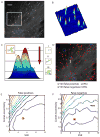
+TIPs mark growing MT plus ends. (A) Dual-channel image of tdTomato-EB3 (red) and GFP-tubulin (green) taken with a spinning-disk confocal microscope (courtesy of Ken Myers, NIH/NHLBI). Bar, 10μm. (B) +TIPs have a higher binding affinity for growing MT plus ends than for the MT lattice, leading to the comet-like appearance observed in fluorescence images like (A). (C) plusTipTracker first tracks +TIP comets (red ovals) to form growth sub-tracks (I, III, V; solid black lines) and subsequently groups sub-tracks inferred to have come from the same MT to reconstruct shrinkage (II; dashed black line) and pause (IV; dashed black line) behavior. Transparent red ovals indicate newly-formed comets. The time lag between MT rescue and reappearance of a detectable comet can lead to underestimation of shrinkage speed and positional drift during pause.

Figure 2

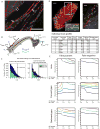
plusTipTracker user interfaces. (A) Interface for project setup, detection, tracking, and post-processing steps of analysis. Red box indicates a blow-up of the interface to the detection algorithm. As a default the software operates with a watershed-based comet detection (see Methods). (B) Interface for various types of track visualization and further analysis, including: interactive track overlays (‘Track Overlays’); movies of regions or individual tracks (‘Track Movies’); movies of tracked comets color-coded by speed (‘Speed Movies’); sub-cellular region-of-interest selection (‘Sub-ROIs’); and MT subpopulation analysis (‘Quadrant Scatter Plots’). See (Applegate and Danuser, 2010) for details.

Figure 3

Particle detection by watershed-based method. (A) Raw image of EGFP-EB3. Bar, 5μm. (B) Intensity landscape of the Difference-of-Gaussian image derived from the white-framed inset shown in (A). (C) Idealized intensity landscape illustrating detection algorithm. Decreasing thresholds, represented by the three horizontal lines crossing the peaks, generate the peak contours shown in panels (i), (ii), and (iii). The contours for peaks 1 and 2 are retained from the middle threshold, while the contour from peak 3 is retained from the lowest threshold. The final detection result is shown in the red-framed inset. (D) Manual (blue) and automatic (red) detection of particles from the image in (A). False positive (yellow) and false negative (cyan) rates are 100(1–99/102) = 2.9% and 100(1–99/103) = 3.9%, respectively (see text for formula details). (E,F) False positive and false negative detections, as a function of the comet signal-to-noise ratio (SNR, defined as amplitude of comet signal divided by standard deviation of the background intensity) and comet eccentricity. Red asterisks indicate the parameter settings used to generate Supplementary Movie 2.

Figure 4

Particle detection by anisotropic Gaussian model fitting method. (A) User interface to the detection algorithm when the option ‘Gaussian fit’ is selected. See Methods for an explanation of the parameters. (B,C) Comparison of the performance of the watershed method and the anisotropic Gaussian model fitting method in detecting particles representing substantially elongated comets. The watershed method tends to detect multiple particles per comet, while anistropic Gaussian model fitting explicitly takes into account the anisotropy of the signal. Detection performance on the entire time-lapse sequence is illustrated in Supplementary Movie 3.

Figure 5

Tracking and inference of complete MT plus-end trajectories. (A) Sub-tracks, which are generated by linking +TIP comets and which indicate the growth of MTs, are unidirectional and often collinear (arrow pairs). Pairs of collinear growth sub-tracks may become candidates for sub-track linking. Bar, 5μm. (B) Illustration of the candidate selection for sub-track linking. Sub-track i (black) starts at t = 0 and ends at t = 8. Candidate sub-tracks j (blue and green) for linking to sub-track i must initiate in the gray search region and start within Δt_max frames (user input to the tracking software) from the end-point of sub-track i. Candidates chosen from the light gray region will generate inferred shrinkage events (blue), while candidates chosen from the dark gray region will generate inferred pause or continuation-of-growth events (green; the latter arises due to detection failure or the comet moving temporarily out of focus). The cost of linking depends on the time gap between the sub-track end and candidate start, Δt_gap, and the three spatial parameters d_||, d_⊥, θ. See text for details of these parameters and the cost function. (C) The cost of sub-track linking is directionally unbiased, as shown by the distribution of costs in the forward (green) and backward (blue) directions for all potential links (left). For tracks with only one candidate, the balance is maintained (right). Sub-track pairs with costs higher than the death cost (vertical line) will not be chosen for linking, allowing proper termination of trajectories where pause or shrinkage is unlikely. (D) The ‘Track Overlays’ tool (Figure 2B) was used to show all tracks on the image (left; bar, 10μm), zoom in, select an individual track (right; bar, 5μm) from the hundreds shown in the inset, and view its profile (table). In this example profile the lifetimes and displacements are reported in seconds and microns, while the software returns them in frames and pixels. This track corresponds to Supplementary Movie 4. (E) Evaluation of frame-to-frame and sub-track linking (forward and backward gaps separated) in simulated +TIP movies.

Figure 6

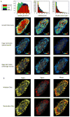
Spatial maps of MT dynamics. (A) Top row: stacked speed, lifetime, and displacement distributions for growth, fgap, and bgap sub-tracks. Rows 2–4: growth, fgap, and bgap sub-tracks color-coded by speed (left column), lifetime (center column), and displacement (right column). Bar, 10μm. (B) Initiation (top row) and termination (bottom row) sites for fgaps (left) and bgaps (right). Merged images are shown in the right column. The merged distributions of fgap and bgap initiations/termination sites are equivalent to the distributions of termination/initiation sites of growth events participating in compound trajectories.

Figure 7

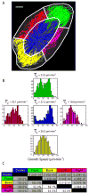
Sub-cellular organization of growth speed. (A) Using the ‘Sub-ROIs’ tool (Figure 2B), growth sub-tracks were extracted from five regions of the cell (center, blue; front, green; back, yellow; left, red; right, magenta). Bar, 10μm. (B) Growth speed distributions for the five regions. (C) Discrimination matrix containing the results of two statistical tests for each pair of cell regions. Below the diagonal: percent confidence that the distributions are different, from a bootstrapped, mean-subtracted Kolmogorov-Smirnov test. Above the diagonal: p-values for a permutation t-test of the means. Significant differences shown in gray.

Figure 8

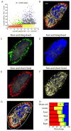
Proportions of MT subpopulations classified by growth speed and growth lifetime. (A) The ‘Quadrant Scatter Plot’ tool (Figure 2B) was used to generate a speed vs. lifetime scatter plot split into quadrants based on mean growth speed (21.7μm·min⁻¹; corresponding to the 49th percentile) and mean growth lifetime (12.9s; corresponding to the 66th percentile), generating four distinct subpopulations of growth sub-tracks. (B) Sub-tracks corresponding to the data points in (A) are overlaid together on the image with the same color scheme to show relative spatial arrangement. The four subpopulations thus represent slow and long-lived (C), fast and long-lived (D), slow and short-lived (E), and fast and short-lived growth events. Growth sub-tracks extracted from the sub-ROIs used in Figure 7(G) show the relative proportions of the subpopulations in different sub-cellular regions (H).

Figure 9

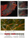
Evaluation of plusTipTracker performance on two-color dataset. (A) Overlay of plusTipTracker results on EB1-EGFP image. (B) Growth tracks obtained by manual and automatic tracking overlaid on mCherry-tubulin image corresponding to inset in (A). (C) Visual comparison of manual (left) and automatic (right) tracks for a single MT (No. 1 in the annotated list; see Supplementary Excel file), overlaid on two-color merged image. Blue crosses represent hand-tracked comet positions. (D) Annotated track profiles describing sources of variation in manual and automatic tracking results.

References

1. Akhmanova A, Hoogenraad CC. Microtubule plus-end-tracking proteins: mechanisms and functions. Current Opinion in Cell Biology. 2005;17:47–54. - PubMed
1. Alberts B, Johnson A, Lewis J, Raff M, Roberts K, et al. Molecular biology of the cell. 4. Garland Science; New York: 2002.
1. Applegate KT, Danuser G. Technical Report: Using the plusTipTracker Software to Measure and Analyze Microtubule Dynamics from +TIP Comets. 2010 Accompanying software release ( lccb.hms.harvard.edu/software)
1. Bieling P, Laan L, Schek H, Munteanu EL, Sandblad L, et al. Reconstitution of a microtubule plus-end tracking system in vitro. Nature. 2007;450:1100–1105. - PubMed
1. Burkard KE, Cela E. Linear Assignment Problems and Extensions. In: Du DZ, Pardalos PM, editors. Handbook of Combinatorial Optimization - Supplement Volume A. Supp A. Kluwer Academic Publishers; Dordrecht, NL: 1999. pp. 75–149.pp. 75–149.
Publication types
Substances
LinkOut - more resources