Representation of vestibular and visual cues to self-motion in ventral intraparietal cortex

Abstract

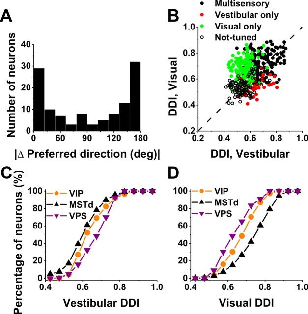
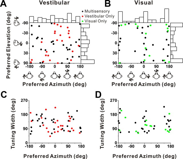
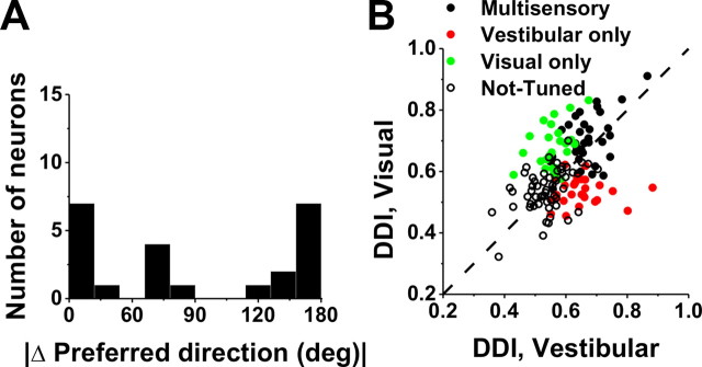
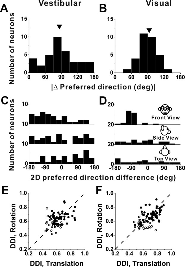
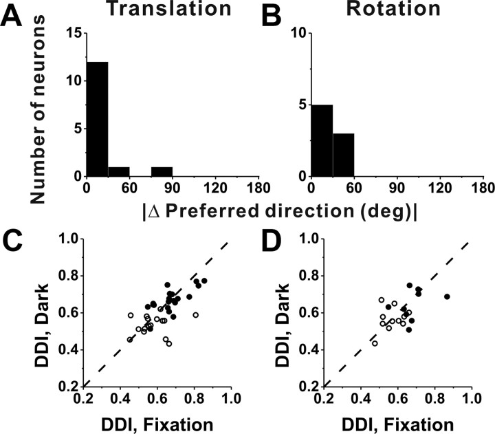
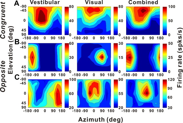
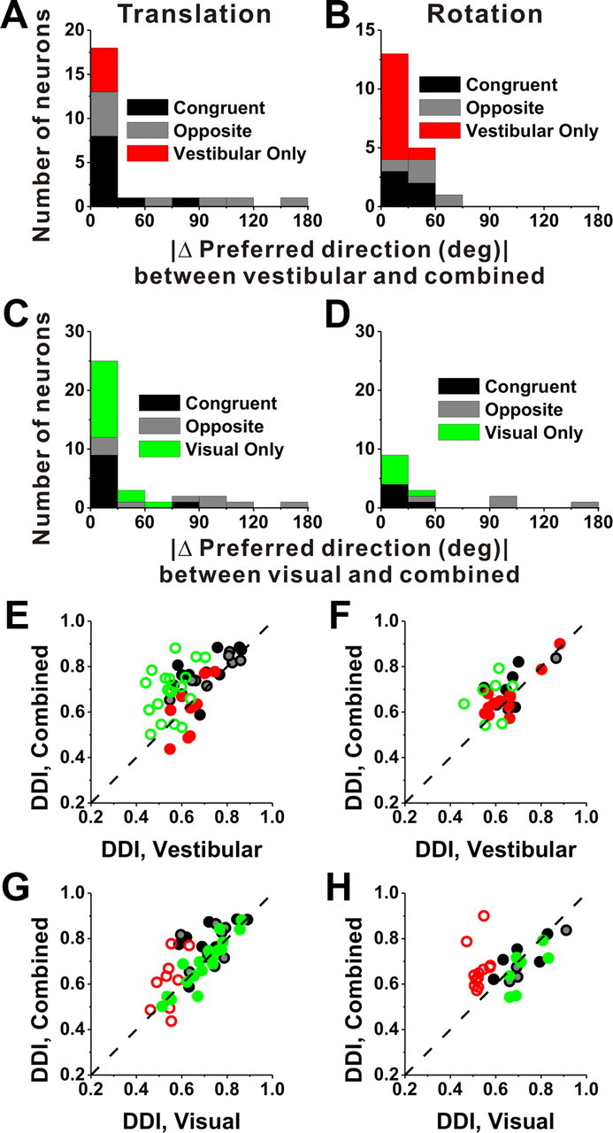
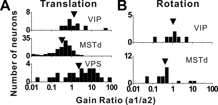
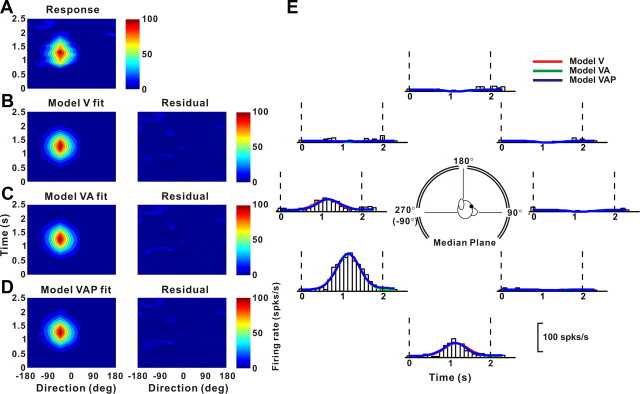
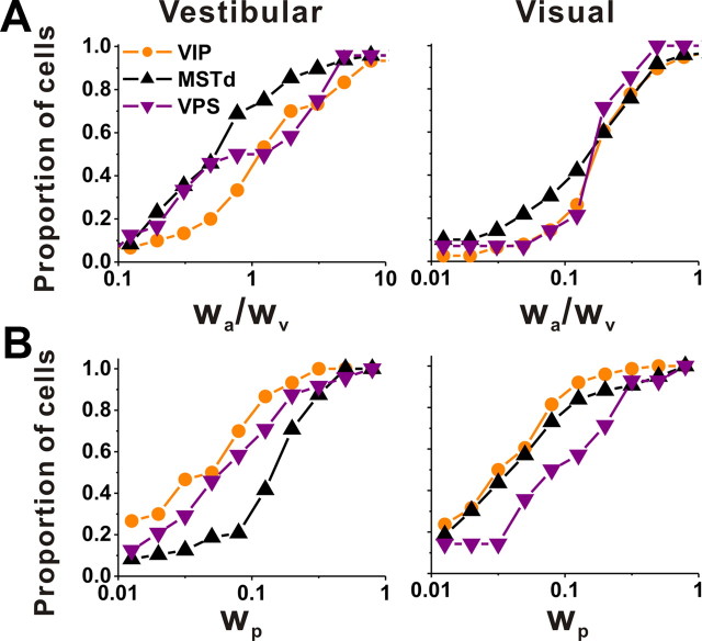
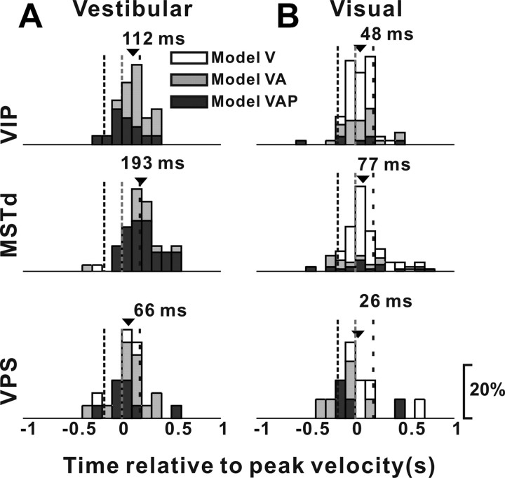
Convergence of vestibular and visual motion information is important for self-motion perception. One cortical area that combines vestibular and optic flow signals is the ventral intraparietal area (VIP). We characterized unisensory and multisensory responses of macaque VIP neurons to translations and rotations in three dimensions. Approximately one-half of VIP cells show significant directional selectivity in response to optic flow, one-half show tuning to vestibular stimuli, and one-third show multisensory responses. Visual and vestibular direction preferences of multisensory VIP neurons could be congruent or opposite. When visual and vestibular stimuli were combined, VIP responses could be dominated by either input, unlike the medial superior temporal area (MSTd) where optic flow tuning typically dominates or the visual posterior sylvian area (VPS) where vestibular tuning dominates. Optic flow selectivity in VIP was weaker than in MSTd but stronger than in VPS. In contrast, vestibular tuning for translation was strongest in VPS, intermediate in VIP, and weakest in MSTd. To characterize response dynamics, direction-time data were fit with a spatiotemporal model in which temporal responses were modeled as weighted sums of velocity, acceleration, and position components. Vestibular responses in VIP reflected balanced contributions of velocity and acceleration, whereas visual responses were dominated by velocity. Timing of vestibular responses in VIP was significantly faster than in MSTd, whereas timing of optic flow responses did not differ significantly among areas. These findings suggest that VIP may be proximal to MSTd in terms of vestibular processing but hierarchically similar to MSTd in terms of optic flow processing.

Figure 1.

Anatomical localization of recording sites. A, Inflated cortical surface illustrating the locations of the coronal sections drawn in B–G. B–D, Coronal sections from both hemispheres of monkey J, spaced 4 mm apart, are shown from posterior (B) to anterior (D). E–G, Coronal sections from the right hemisphere of monkey C are shown from posterior (E) to anterior (G). Cells located within 2 mm of each section were projected onto that section. The black symbols represent single units with significant tuning to either vestibular or visual translation. The white symbols represent cells that showed no directional tuning.

Figure 2.

Stimuli and examples of 3D translation tuning. A, Schematic of the 26 movement trajectories in 3D, spaced 45° apart in both azimuth and elevation. B, The 2 s translational motion stimulus: velocity (blue), acceleration (green), and position (magenta). C, Response PSTHs (left panels) and 3D tuning profiles (right panels) for a congruent VIP neuron. The red line indicates the peak time (t_vestibular = 1.04; t_visual = 0.91 s) when the maximum response across directions occurred. The 3D tuning profile (right) is illustrated as a color contour map (Lambert cylindrical projection), taken at the peak response time (vestibular DDI, 0.77; visual DDI, 0.87). Tuning curves along the margins of the color map illustrate mean firing rates plotted versus elevation or azimuth (averaged across azimuth or elevation, respectively). The preferred directions for this cell (computed as vector sum) are [azimuth, elevation] = [−24, −38°] for the vestibular condition, and [−6, −64°] for the visual condition. D, PSTHs and spatial tuning profile for a VIP neuron with opposite direction preferences in the vestibular ([azimuth, elevation] = [−64, 7°]; DDI, 0.64; peak time, 0.94 s) and visual conditions ([129, 7°]; DDI, 0.75; peak time, 1.06 s).

Figure 3.

Example of a VIP neuron with double-peaked direction tuning in the vestibular condition. A, B, PSTHs for 26 directions during presentation of vestibular (A) and visual (B) translation stimuli. The red and green lines indicate the two peak times for the vestibular translation response (t_vestibular = 0.91 and 1.41 s). Note that there was only one peak time for the visual response (t_visual = 0.96 s; red). C, D, The 3D directional tuning for the vestibular condition is illustrated at each of the two peak times. At the first peak time (C), the direction preference is [azimuth, elevation] = [39, −16°], and the DDI is 0.84; at the second peak time (D), the direction preference is [−126, 9°], and the vestibular DDI is 0.78. E, Three-dimensional directional tuning for the visual condition. The preferred direction is [−168, 12°], and the visual DDI is 0.79.

Figure 4.

Summary of direction tuning properties of VIP neurons during translation. A, B, Distribution of vestibular (A) and visual (B) 3D heading preferences. Each data point in the scatter plot corresponds to the preferred azimuth (abscissa) and elevation (ordinate) of a single neuron with significant unimodal heading tuning (A, n = 184; B, n = 240). The data are plotted on Cartesian axes that represent the Lambert cylindrical equal-area projection of the spherical stimulus space. Histograms along the top and right sides of each scatter plot show the marginal distributions. The dashed elliptical curves represent a ±30° range of directions around straight forward ([azimuth, elevation] = [90, 0°]) and straight backward ([azimuth, elevation] = [−90, 0°]). C, D, Scatter plots of the tuning width at half-maximum of each cell, computed from the tuning curve in the horizontal plane, versus preferred azimuth. The black dots represent cells with significant unimodal spatial tuning during both the vestibular (n = 149) and visual (n = 141) conditions. The red dots represent cells with significant unimodal vestibular tuning only (n = 35). The green dots represent cells with significant unimodal visual tuning only (n = 99).

Figure 5.

Comparison of tuning preferences and direction selectivity between visual and vestibular responses of VIP neurons during translation. A, Distribution of the absolute difference in 3D preferred direction (|Δ preferred direction|) between visual and vestibular responses (n = 118). Note that bins were computed according to the cosine of the angle (in accordance with the spherical nature of the data, such that the distribution would be flat if there were no systematic relationship between visual and vestibular direction preferences). Only neurons with significant unimodal spatial tuning during both vestibular and visual conditions have been included. B, Scatter plot of the visual DDI as a function of the vestibular DDI. Black filled symbols, Cells with significant tuning during both the vestibular and visual conditions (n = 182); red symbols, cells with significant tuning during the vestibular condition only (n = 40); green symbols, cells with significant tuning during the visual condition only (n = 128); open symbols, cells without significant tuning in either condition (n = 102). Dashed line, Unity-slope diagonal. C, Cumulative distributions of DDI for vestibular responses to translation in VIP (orange; n = 452), MSTd (black; n = 336), and VPS (purple; n = 166). D, Cumulative distributions of DDI for visual responses.

Figure 6.

Summary of tuning properties of VIP neurons during rotation. A, B, Distribution of vestibular (A) and visual (B) 3D rotation preferences. Each data point in the scatter plot corresponds to the preferred azimuth (abscissa) and elevation (ordinate) of a single neuron with significant unimodal heading tuning (A, n = 53; B, n = 43). The format is as in Figure 4. C, D, Scatter plots of the tuning width at half-maximum of each cell versus preferred azimuth. The black symbols represent cells with significant unimodal tuning during both the vestibular (n = 31) and visual (n = 28) conditions. The red symbols represent cells with significant unimodal vestibular tuning only (n = 22). The green symbols represent cells with significant unimodal visual tuning only (n = 15).

Figure 7.

Comparison of tuning preferences and direction selectivity between visual and vestibular responses of VIP neurons during rotation. A, Distribution of the absolute 3D difference in preferred direction (|Δ preferred direction|) between visual and vestibular responses (n = 23). The format is as in Figure 5. Only neurons with significant unimodal spatial tuning during both vestibular and visual conditions have been included. B, Scatter plot of the visual DDI as a function of the vestibular DDI. Black filled symbols, with significant tuning during both the vestibular and visual conditions (n = 36); red symbols, cells with significant tuning during the vestibular condition only (n = 27); green symbols, cells with significant tuning during the visual condition only (n = 24); open symbols, cells without significant tuning in either condition (n = 55). Dashed line, Unity-slope diagonal.

Figure 8.

Summary of differences in direction preference and tuning strength between rotation and translation. A, B, Histograms of the absolute differences in 3D preferred direction (|Δ preferred direction|) between rotation and translation for the vestibular (n = 36) and visual (n = 32) conditions, respectively (calculated only for neurons with significant unimodal tuning in both conditions). The arrows illustrate mean values. C, D, Distributions of preferred direction differences projected onto each of the three cardinal planes: frontoparallel (front view), sagittal (side view), and horizontal (top view). E, F, Scatter plots of the rotation and translation DDI values for the vestibular and visual conditions, respectively. The filled symbols indicate cells with significant tuning for both rotation and translation (ANOVA, p < 0.01) (E, n = 45; F, n = 55); the open symbols denote cells without significant tuning for either one or both of the rotation and translation protocols (ANOVA, p > 0.01) (E, n = 37; F, n = 27). Dashed lines, Unity-slope diagonals.

Figure 9.

Comparison between VIP responses during fixation and in darkness. A, B, Distribution of the absolute difference in preferred direction for neurons with significant unimodal tuning during both fixation and in complete darkness; data are shown for translation (A) (n = 14) and rotation (B) (n = 8) separately. C, D, Scatter plot of DDI values for cells tested in both fixation and darkness conditions during translation (C) (n = 36) and rotation (D) (n = 20). Filled symbols, Cells with significant spatial tuning during both fixation and darkness (C, n = 20; D, n = 9). Open symbols, Cells without significant spatial tuning during either fixation or total darkness (C, n = 16; D, n = 11). Dashed lines, Unity-slope diagonals.

Figure 10.

Examples of 3D translation tuning for three VIP neurons tested in the vestibular (left), visual (middle), and combined (right) conditions. The format is as in Figure 2. A, Tuning of a congruent multisensory neuron. Vestibular condition: Direction preference, [−40, −55°]; DDI, 0.85; visual condition: direction preference, [−32, −73°]; DDI, 0.84; combined condition: direction preference, [−31, −61°]; DDI, 0.88. B, Tuning of an opposite multisensory neuron for which the combined direction preference was dominated by the vestibular input. Vestibular condition: Direction preference, [−149, 0°]; DDI, 0.86; visual condition: direction preference, [88, −17°]; DDI, 0.78; combined condition: direction preference, [−159, −1°]; DDI, 0.83. C, Tuning of an opposite multisensory neuron for which the combined preference was dominated by the visual input. Vestibular condition: [136, 23°]; DDI, 0.55; visual condition: direction preference, [−6, −31°]; DDI, 0.63; combined condition: direction preference, [26, −19°]; DDI, 0.65.

Figure 11.

Summary of the differences in direction preference and comparison of tuning strength between the combined condition and each of the vestibular and visual conditions. A, B, Distributions of the absolute difference in 3D preferred direction (|Δ preferred direction|) between the combined condition and the vestibular condition, for responses obtained during translation (A) and rotation (B). C, D, Distributions of |Δ preferred direction| between the combined condition and the visual condition, for both translation (C) and rotation (D). E–H, Scatter plots comparing the combined DDI against either the vestibular or the visual DDI. Filled symbols, Cells for which both the combined and vestibular (E, G) or visual (F, H) tuning was significant (ANOVA, p < 0.01). Open symbols, for which either the combined and/or the vestibular/visual tuning was not significant (ANOVA, p > 0.01). Black symbols/bars, Multisensory congruent neurons (E, G, n = 10; F, H, n = 5); gray symbols/bars, multisensory opposite neurons (E, G, n = 9; F, H, n = 4); red symbols/bars, vestibular-only neurons (E, G, n = 9; F, H, n = 12); green symbols/bars, visual-only neurons (E, G, n = 19; F, H, n = 7). Dashed line, Unity-slope diagonal.

Figure 12.

Distributions of the gain ratio, describing the relative weighting of the visual and vestibular contributions to the combined response for translation (A) and rotation (B). A, Top row, Data from area VIP (n = 17); middle row, data from area MSTd (n = 125); bottom row, data from area VPS (n = 26). The arrows illustrate geometric mean values. B, Top row, Data from VIP (n = 7); bottom row, data from area MSTd (n = 19). Only data with significant spatial tuning for both visual and vestibular stimuli and with good fits of the linear model (R² > 0.7) are included in this analysis.

Figure 13.

Example fits of velocity (model V), velocity plus acceleration (model VA), and velocity plus acceleration plus position (model VAP) models to the spatiotemporal visual responses of a VIP neuron. A, Direction–time plot showing how direction tuning evolves over the time course of the response (spatial and temporal resolution, 45° and 100 ms, respectively). B–D, Model fits (left) and response residuals (right). For model V (B), t₀ = 1.042 s; θ = −43.2°, R² = 0.934. For model VA (C), t₀ = 1.148 s; θ₀ = −43.3°, Δθ_va = 5.9°, w_v = 0.825, R² = 0.935. For model VAP (D), t₀ = 1.149 s; θ₀ = −43.3°, Δθ_va = 5.5°, w_v = 0.81, Δθ_vp = 5.5°, w_p = 0.031, R² = 0.936. E, Response PSTHs (open bars) for the eight directions of motion in the median plane (see inset) along with superimposed fits of model V (red), model VA (green), and model VAP (blue). The vertical dashed lines mark the 2 s duration of the stimulus.

Figure 14.

Population comparison of parameters of spatiotemporal model fits among VIP, MSTd, and VPS. A, Cumulative distributions of the ratio of acceleration to velocity weights (w_a/w_v) from model VA for the vestibular (left, VIP, n = 30; MSTd, n = 48; VPS, n = 24) and visual (right, VIP, n = 76; MSTd, n = 119; VPS, n = 14) conditions. B, Cumulative distributions of the position weight, w_p, from model VAP for the vestibular (left, VIP, n = 30; MSTd, n = 48; VPS, n = 24) and visual (right, VIP, n = 76; MSTd, n = 119; VPS, n = 14) conditions. Only data with good fits (R² > 0.7) were included here.

Figure 15.

Distributions of response latency, derived from model fits, for neurons in VIP (top row), MSTd (middle row), and VPS (bottom row), as tested under the vestibular (A, VIP, n = 30; MSTd, n = 48; VPS, n = 24) and visual (B, VIP, n = 76; MSTd, n = 119; VPS, n = 14) conditions. Open bars, Cells better fit with model V; gray bars, cells better fit with model VA; black bars, cells better fit with model VAP. The arrows indicate mean values. The vertical dashed lines indicate the times of peak acceleration/deceleration and peak velocity of the stimulus.

Figure 16.

Relationship between tuning strength, as measured by DDI, and cell location within the intraparietal sulcus. DDI values for the vestibular condition (top row) and the visual condition (bottom row) are plotted as a function of the anterior–posterior stereotaxic coordinate of each electrode penetration (shown in millimeters, with 0 mm corresponding to AP-0). A, Data recorded from the left hemisphere (LH) of monkey J (left column, n = 53) and the right hemisphere (RH) of monkey J (right column, n = 70). B, Data obtained from the right hemisphere of monkey C (n = 112). Black symbols, Multisensory neurons; red symbols, vestibular-only neurons; green symbols, visual-only neurons. The solid lines illustrate the best-fit lines from linear regressions. Note that only responsive cells are included in these scatter plots. “+” marks the mean location for each group of cells.

References

1. Angelaki DE, Cullen KE. Vestibular system: the many facets of a multimodal sense. Annu Rev Neurosci. 2008;31:125–150. - PubMed
1. Anzai A, Peng X, Van Essen DC. Neurons in monkey visual area V2 encode combinations of orientations. Nat Neurosci. 2007;10:1313–1321. - PubMed
1. Avillac M, Denève S, Olivier E, Pouget A, Duhamel JR. Reference frames for representing visual and tactile locations in parietal cortex. Nat Neurosci. 2005;8:941–949. - PubMed
1. Avillac M, Ben Hamed S, Duhamel JR. Multisensory integration in the ventral intraparietal area of the macaque monkey. J Neurosci. 2007;27:1922–1932. - PMC - PubMed
1. Baizer JS, Ungerleider LG, Desimone R. Organization of visual inputs to the inferior temporal and posterior parietal cortex in macaques. J Neurosci. 1991;11:168–190. - PMC - PubMed
Publication types
LinkOut - more resources