

Systematic clustering of transcription start site landscapes
- PMID: 21887249
- PMCID: PMC3160847
- DOI: 10.1371/journal.pone.0023409
Systematic clustering of transcription start site landscapes
Abstract
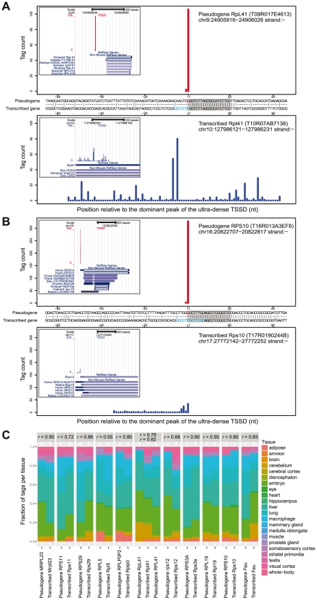
Genome-wide, high-throughput methods for transcription start site (TSS) detection have shown that most promoters have an array of neighboring TSSs where some are used more than others, forming a distribution of initiation propensities. TSS distributions (TSSDs) vary widely between promoters and earlier studies have shown that the TSSDs have biological implications in both regulation and function. However, no systematic study has been made to explore how many types of TSSDs and by extension core promoters exist and to understand which biological features distinguish them. In this study, we developed a new non-parametric dissimilarity measure and clustering approach to explore the similarities and stabilities of clusters of TSSDs. Previous studies have used arbitrary thresholds to arrive at two general classes: broad and sharp. We demonstrated that in addition to the previous broad/sharp dichotomy an additional category of promoters exists. Unlike typical TATA-driven sharp TSSDs where the TSS position can vary a few nucleotides, in this category virtually all TSSs originate from the same genomic position. These promoters lack epigenetic signatures of typical mRNA promoters and a substantial subset of them are mapping upstream of ribosomal protein pseudogenes. We present evidence that these are likely mapping errors, which have confounded earlier analyses, due to the high similarity of ribosomal gene promoters in combination with known G addition bias in the CAGE libraries. Thus, previous two-class separations of promoter based on TSS distributions are motivated, but the ultra-sharp TSS distributions will confound downstream analyses if not removed.
Conflict of interest statement
Figures
 ), the next the three cluster partition (
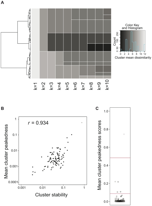
 ), etc. The color intensity indicates the mean dissimilarity between all the TSSDs within one cluster (darker means higher homogeneity). Note that most clusters are inhomogeneous when k is low: clusters with high homogeneity only emerge when moving the cutline closer to the leaves. (B) Correlation between the mean cluster peakedness and the cluster stability. The scatter plot compares the cluster stability scores resulting from the bootstrap resampling to the intra-cluster peakedness scores. R denotes the Pearson's correlation coefficient of the scores (
 ). (C) Distribution of intra-cluster peakedness scores of 500 TSSD clusters generated by hierarchical clustering. The Y-axis shows the intra-cluster peakedness scores. The red lines indicate offsets for defining three larger clusters using k-means. Each box represents one TSSD cluster.

Similar articles
-
Genome-wide identification and characterization of transcription start sites and promoters in the tunicate Ciona intestinalis.Genome Res. 2016 Jan;26(1):140-50. doi: 10.1101/gr.184648.114. Epub 2015 Dec 14. Genome Res. 2016. PMID: 26668163 Free PMC article.
-
Genome-wide analysis of core promoter structures in Schizosaccharomyces pombe with DeepCAGE.RNA Biol. 2015;12(5):525-37. doi: 10.1080/15476286.2015.1022704. RNA Biol. 2015. PMID: 25747261 Free PMC article.
-
TSS seq based core promoter architecture in blood feeding Tsetse fly (Glossina morsitans morsitans) vector of Trypanosomiasis.BMC Genomics. 2015 Sep 22;16(1):722. doi: 10.1186/s12864-015-1921-6. BMC Genomics. 2015. PMID: 26394619 Free PMC article.
-
Genomic and chromatin signals underlying transcription start-site selection.Trends Genet. 2011 Nov;27(11):475-85. doi: 10.1016/j.tig.2011.08.001. Epub 2011 Sep 15. Trends Genet. 2011. PMID: 21924514 Review.
-
Role of DNA sequence based structural features of promoters in transcription initiation and gene expression.Curr Opin Struct Biol. 2014 Apr;25:77-85. doi: 10.1016/j.sbi.2014.01.007. Epub 2014 Feb 4. Curr Opin Struct Biol. 2014. PMID: 24503515 Review.
Cited by
-
Identifying transcript 5' capped ends in Plasmodium falciparum.PeerJ. 2021 Aug 25;9:e11983. doi: 10.7717/peerj.11983. eCollection 2021. PeerJ. 2021. PMID: 34527439 Free PMC article.
-
DNMT and HDAC inhibitors induce cryptic transcription start sites encoded in long terminal repeats.Nat Genet. 2017 Jul;49(7):1052-1060. doi: 10.1038/ng.3889. Epub 2017 Jun 12. Nat Genet. 2017. PMID: 28604729 Free PMC article.
-
VprBP/DCAF1 triggers melanomagenic gene silencing through histone H2A phosphorylation.Res Sq [Preprint]. 2023 Jul 12:rs.3.rs-2950076. doi: 10.21203/rs.3.rs-2950076/v2. Res Sq. 2023. Update in: Biomedicines. 2023 Sep 17;11(9):2552. doi: 10.3390/biomedicines11092552. PMID: 37293029 Free PMC article. Updated. Preprint.
-
Trends in disease burden of hepatitis B infection in Jiangsu Province, China, 1990-2021.Infect Dis Model. 2023 Jul 10;8(3):832-841. doi: 10.1016/j.idm.2023.07.007. eCollection 2023 Sep. Infect Dis Model. 2023. PMID: 37520113 Free PMC article.
-
MMP-9-dependent proteolysis of the histone H3 N-terminal tail: a critical epigenetic step in driving oncogenic transcription and colon tumorigenesis.Mol Oncol. 2024 Aug;18(8):2001-2019. doi: 10.1002/1878-0261.13652. Epub 2024 Apr 10. Mol Oncol. 2024. PMID: 38600695 Free PMC article.
References
-
- Smale ST, Kadonaga JT. The RNA polymerase II core promoter. Annu Rev Biochem. 2003;72:449–479. - PubMed
-
- Carninci P, Kasukawa T, Katayama S, Gough J, Frith MC, et al. The transcriptional landscape of the mammalian genome. Science. 2005;309:1559–1563. - PubMed
-
- Maruyama K, Sugano S. Oligo-capping: a simple method to replace the cap structure of eukaryotic mRNAs with oligoribonucleotides. Gene. 1994;138:171–174. - PubMed
Publication types
MeSH terms
Substances
LinkOut - more resources
Full Text Sources
Other Literature Sources
Molecular Biology Databases
