Fitness landscapes: an alternative theory for the dominance of mutation

Abstract

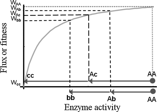
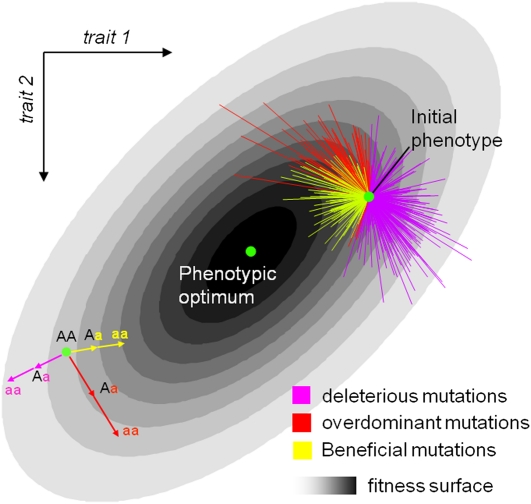
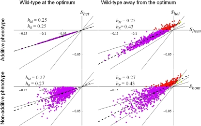
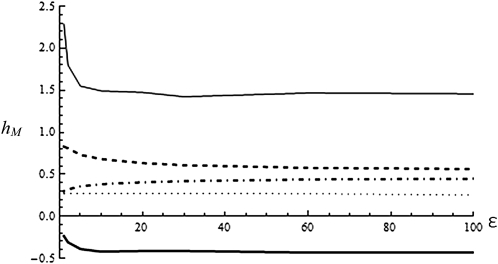
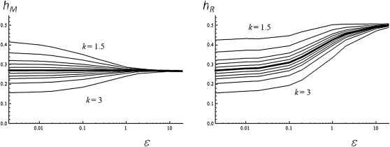
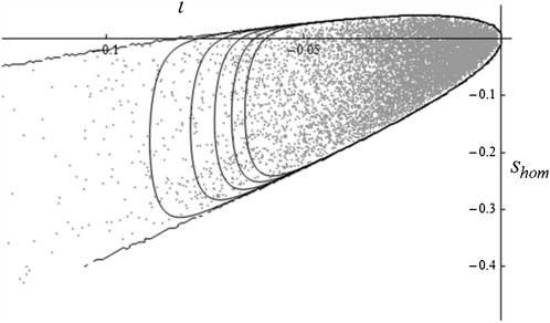
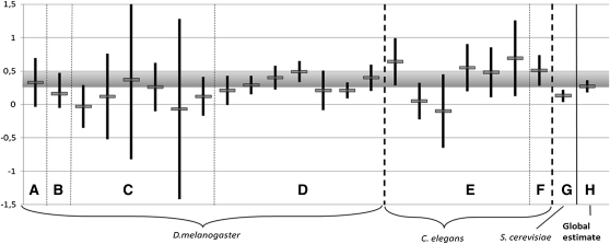
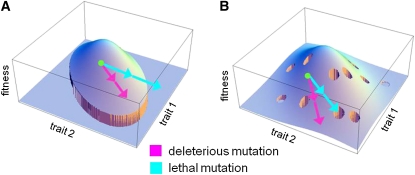
Deleterious mutations tend to be recessive. Several theories, notably those of Fisher (based on selection) and Wright (based on metabolism), have been put forward to explain this pattern. Despite a long-lasting debate, the matter remains unresolved. This debate has focused on the average dominance of mutations. However, we also know very little about the distribution of dominance coefficients among mutations, and about its variation across environments. In this article we present a new approach to predicting this distribution. Our approach is based on a phenotypic fitness landscape model. First, we show that under a very broad range of conditions (and environments), the average dominance of mutation of small effects should be approximately one-quarter as long as adaptation of organisms to their environment can be well described by stabilizing selection on an arbitrary set of phenotypic traits. Second, the theory allows predicting the whole distribution of dominance coefficients among mutants. Because it provides quantitative rather than qualitative predictions, this theory can be directly compared to data. We found that its prediction on mean dominance (average dominance close to 0.25) agreed well with the data, based on a meta-analysis of dominance data for mildly deleterious mutations. However, a simple landscape model does not account for the dominance of mutations of large effects and we provide possible extension of the theory for this class of mutations. Because dominance is a central parameter for evolutionary theory, and because these predictions are quantitative, they set the stage for a wide range of applications and further empirical tests.

Figure 1

Dominance of mutations as predicted by the metabolic control theory. A loss-of-function mutation (c) reducing enzymatic activity to 50% (resp. 0%) when heterozygous (resp. homozygous) has a lethal but strongly recessive effect on metabolic flux (or fitness). A mutation decreasing less drastically the activity of the enzyme (b) has a milder and less recessive effect on metabolic flux (or fitness). However, by construction (i) the heterozygous effect of the lethal mutation is larger than that of the nonlethal (W_Ab > W_Ac) and (ii) overdominance cannot occur.

Figure 2

Two-dimensional illustration of the mutation model. This figure illustrates the principle of the model in two dimensions (two traits). The fitness function is a bivariate Gaussian function, which increases toward an optimum with darker gray shading. Mutants are distributed around an initial phenotype or wild type (green spot). The bottom-left sketch explains how dominance on fitness arises even when the phenotype of the heterozygous mutant is halfway between the initial and the homozygous phenotype (additive phenotypes). The top-right sketch shows how a random draw of mutants around an initial phenotype (green spot) generates a distribution of homozygote and heterozygote fitness effects. Any model of stabilizing selection naturally generates dominance for fitness even when mutations act additively on the underlying phenotype. This is due to the concavity of the fitness surface around the optimum. With such a surface, deleterious mutations (purple) tend to be recessive because if a step in one direction is deleterious (i.e., it increases the distance to the optimum), two steps in the same direction necessarily result in more than twice the deleterious effect. The reverse is true for beneficial mutations (yellow) that tend to be dominant. Interestingly, this model also predicts that some mutations (red) should exhibit overdominance in their fitness effect if mutations that bring the phenotype close to the optimum in one step overshoot it in two steps in the same direction.

Figure 3

Sketch of the behavior of h_R (line) and h_M (thick cross) to measurement of noise and missing or omitted data. (A) All data, thick cross, ratio of means; line, regression. (B) Noisier data, the regression slope decreases, the ratio of means is less affected. (C) Missing or omitted large effects (open circles); the ratio of means changes, the regression slope is less affected.

Figure 4

Limited impact of departures from a purely additive model. Ratios average dominance computed with different values of σ_υ², relative to the value computed in the additive case. For illustration, the distribution of υ corresponding to different values of σ_υ² (cases σ_υ² = 0.0012, 0.003, 0.008, 0.02, 0.05 illustrated) are shown in the insets (the distribution are within [0,1]). Bottom line: ratio E(ι)/E(ι)_add. Top line: ratios of h_M/h_{M add} and h_R/h_{R add} when the wild type is as optimum (s_o = 0) (they superpose). Gray line: ratio h_R/h_{R add} when the wild type is not at the optimum (case considered, s_o = 0.06 and E(s_hom) = 0.05).

Figure 5

Heterozygous vs. homozygous fitness effects under different models assumptions. The relationship between homozygous (s_hom, x-axis) and heterozygous (s_het, y-axis) fitness effects of mutations is compared in four situations. Left vs. right: wild type is either at the optimum (s_o = 0, left) or away from it (s_o = 0.06, right). Top vs. bottom: mutation effects on the underlying phenotype are either all additive (top, E(ν) = 1/2, σ_υ = 0) or only additive on average, with a random dominance coefficient (bottom, E(ν) = 1/2, σ_υ² = 0.02, 95% of υ values fall in the range [0.26–0.74]). Dots show the value of (s_hom, s_het) for exact simulations of 1000 mutants, with corresponding values of h_M and h_R given on each graph. The same color code as in Figure 2 is used: purple, deleterious recessive; yellow, dominant beneficial; red, overdominant. The dashed line is the regression of s_het on s_hom, which is undistinguishable from our prediction (h_R and s_het0, Equation 13). The black dot gives E(s_het) and E(s_hom). The three plain lines indicate s_het = s_hom/4, s_het = s_hom/2 and s_het = s_hom. h_M varies little overall, but h_R increases from 1/4 (left) to a value closer to 1/2 (right) when the wild type is far away from the optimum. In the latter situation, overdominant mutations and dominant beneficial mutations are also frequent.

Figure 6

Average dominance for different mutational classes. h_M (y-axis) measured as a function of the scaled distance to the optimum ε. The dotted line (∙∙∙) is the average over all mutation and is constant. The dot-dashed (– ^. –) line indicates h_M for mutations that are deleterious in both heterozygous and homozygous state (purple points on Figure 5). The dashed line (– – –) indicates h_M for mutations that are beneficial in both heterozygous and homozygous state (yellow points on Figure 5). The solid line indicates h_M for mutations that are overdominant, with beneficial (thin line) or deleterious (thick line) homozygous effect (red points on Figure 5). Values obtained by exact simulations with E(ν) = 1/2, σ_υ² = 0.02. Different values of E(s_hom) give undistinguishable curves.

Figure 7

Peakedness of the fitness function. Effect of the peakedness of the fitness function (k, as described in the text) on average dominance (h_M, left; h_R, right) as a function of the scaled distance to the optimum ε = s_o/E(s_hom). The case of a quadratic log-fitness (k = 2) is indicated by the thick line (other k values are from top to bottom: k = 1.5; 1.7; 1.8; 1.9; 2; 2.1; 2.2; 2.3; 2.5; 3). Average measure obtained by simulations (E(s_hom) = 0.05; σ_υ² = 0.02).

Figure 8

Bivariate distribution Φ{ι,s_hom}. Illustration of the bivariate distribution Φ{ι, s_hom}, given in Equation 23 (black lines) with exact simulation of 10,000 mutants (gray dots). Parameter values are s_o = 0.04 and E(s_hom) = 0.05, n_e = 3.5.

Figure 9

Survey of empirical estimates of average dominance. We confronted our prediction (h_R within [0.25–0.5] and closer to 0.25, shaded region) with different empirical estimates of h_R (with their confidence interval), across species and different traits. D. melanogaster: (A) viability (Chavarrias et al. 2001), (B) viability (Fry and Nuzhdin 2003), (C) female early fecundity, female late fecundity, male longevity, female longevity, male mating ability, weighted mean (not used to calculate our composite estimate of average dominance) (Houle et al. 1997), (D) viability, recalculated h_R from different Mukai’s experiments (Simmons and Crow 1977). C. elegans: (E) productivity, survival to maturity, longevity, intrinsic rate of increase, convergence rate, generation rate (Vassilieva et al. 2000), (F) relative fitness (Peters et al. 2003). Saccharomyces cerevisiae, (G) growth rate (Szafraniec et al. 2003). (H) Composite weighted estimate of h_R across studies 0.27 [CI 0.18–0.36].

Figure 10

Alternative models for mutations of large effect and lethals. (A) The fitness function is truncated for extreme trait values: any mutation with effect larger than some fitness threshold has a much stronger deleterious effect than with a smooth landscape model. As a consequence, the average heterozygous effect of mutations of weak homozygous effect (pink) is necessarily smaller than that of mutations of large homozygous (blue). (B) Mutations of large effects and lethals result from genetic incompatibilities unrelated to the trait values. For the sake of illustration, these incompatibilities are illustrated as small random holes on the fitness surface, but these holes are not necessarily a fixed feature of the fitness surface, they may differ across genetic background or environments. In this case the average heterozygous effect of mild and strongly deleterious mutations (including lethal) is equal on average.

References

1. Agrawal A. F., 2009. Spatial heterogeneity and the evolution of sex in diploids. Am. Nat. 174: S54–S70 - PubMed
1. Agrawal A. F., Whitlock M. C., 2011. Inferences about the distribution of dominance drawn from yeast gene knockout data. Genetics 187: 553–566 - PMC - PubMed
1. Bagheri H., Wagner G., 2004. Evolution of dominance in metabolic pathways. Genetics 168: 1713–1735 - PMC - PubMed
1. Barton N. H., 2001. The role of hybridization in evolution. Mol. Ecol. 10: 551–568 - PubMed
1. Bataillon T., Kirkpatrick M., 2000. Inbreeding depression due to mildly deleterious mutations in finite populations: size does matter. Genet. Res. 75: 75–81 - PubMed
Publication types