. 2011 Jul:(158):5-132.

Air toxics exposure from vehicle emissions at a U.S. border crossing: Buffalo Peace Bridge Study

Affiliations

Air toxics exposure from vehicle emissions at a U.S. border crossing: Buffalo Peace Bridge Study

John Spengler et al. Res Rep Health Eff Inst. 2011 Jul.

Abstract

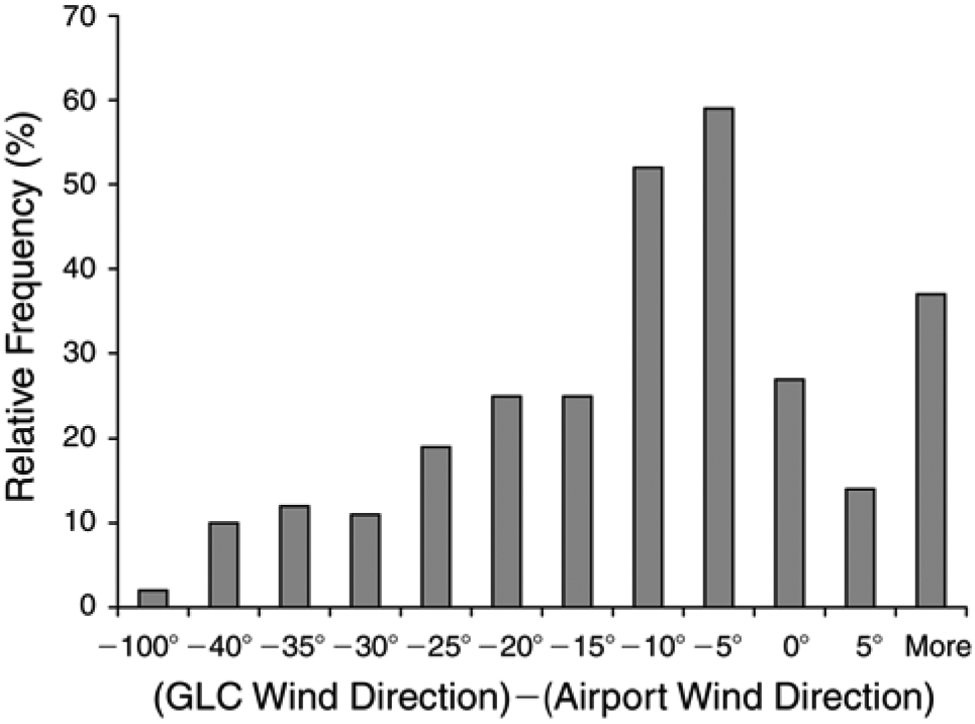
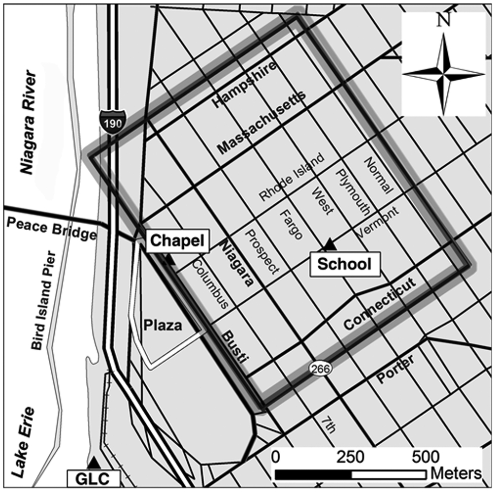
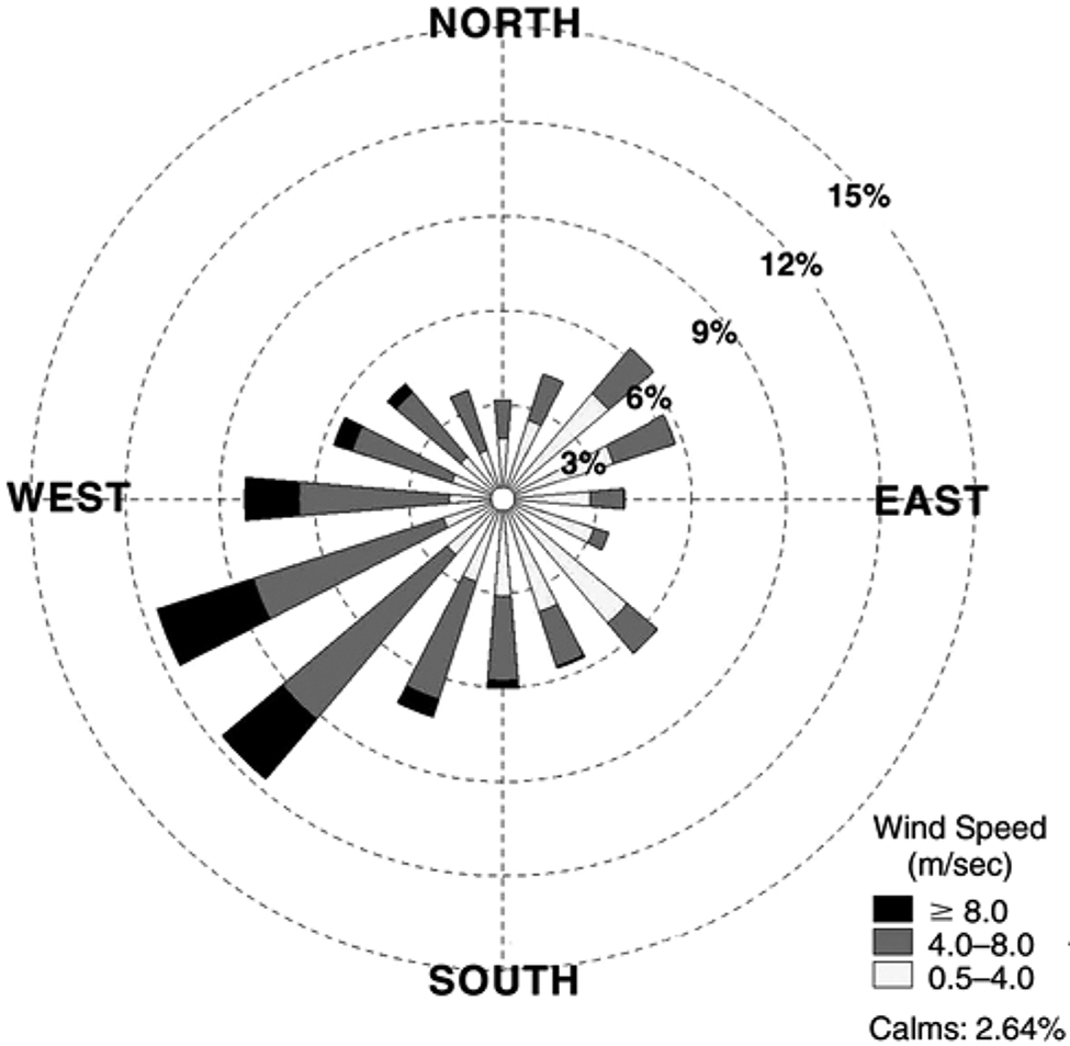
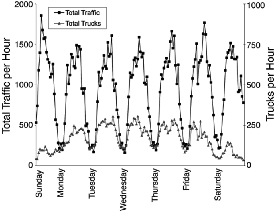
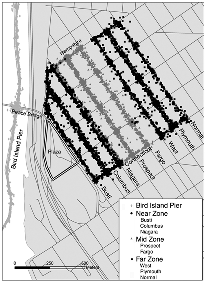
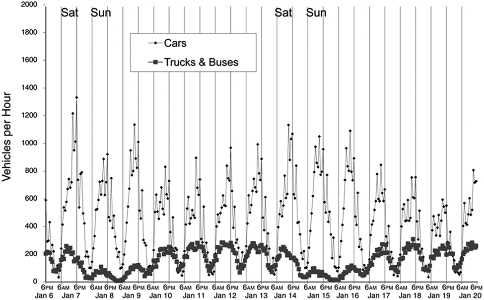
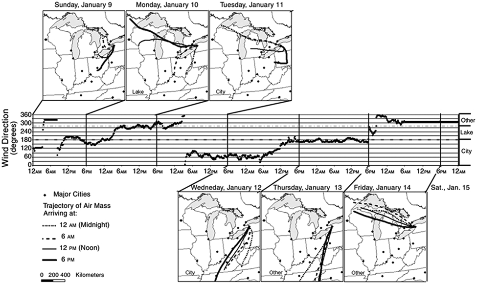
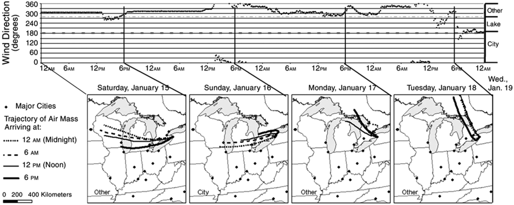
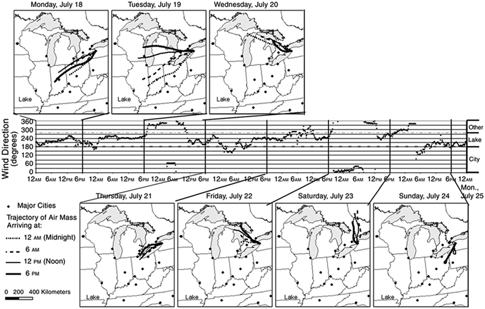
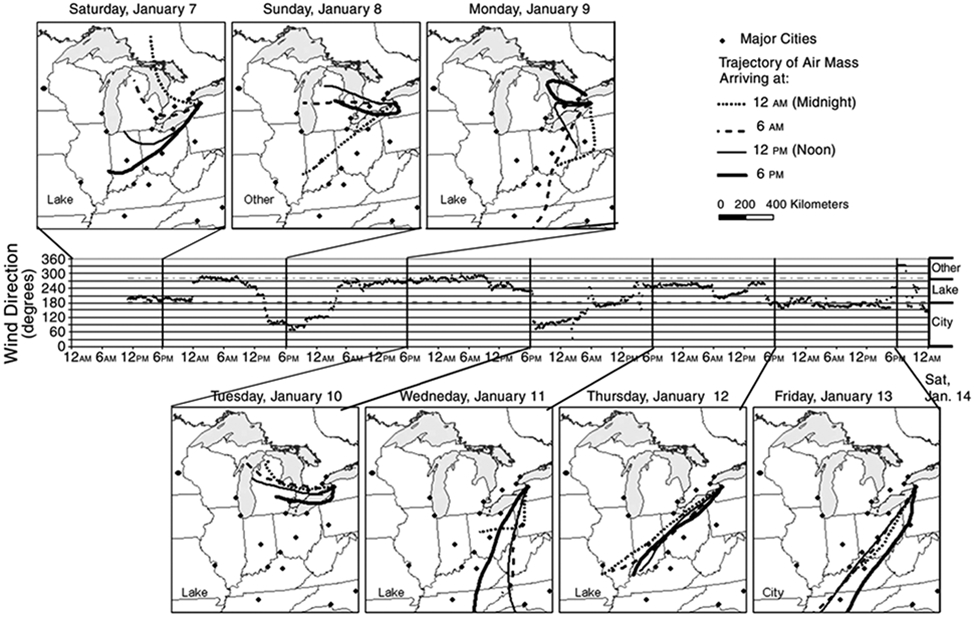
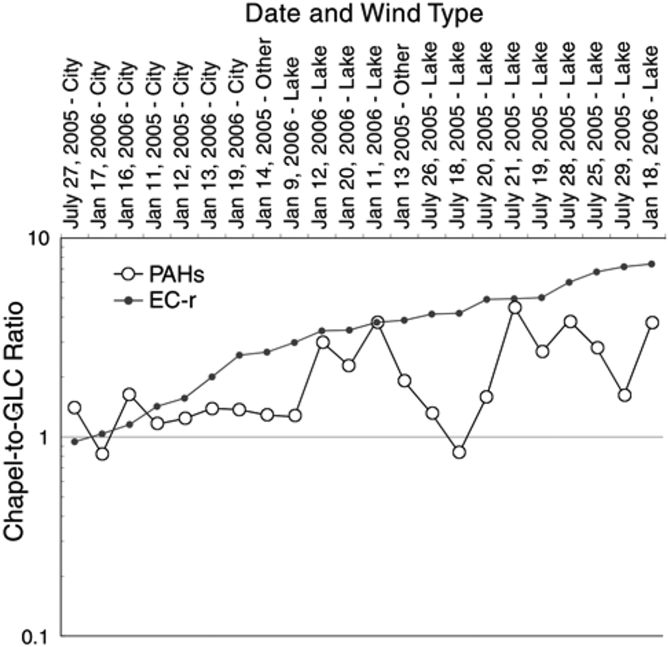
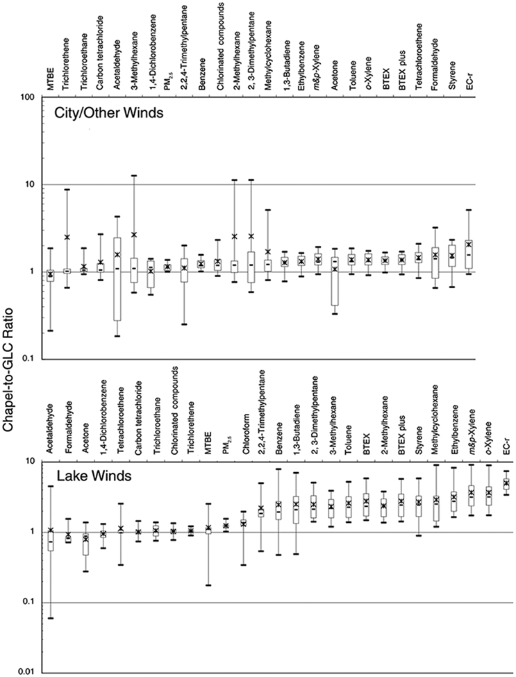
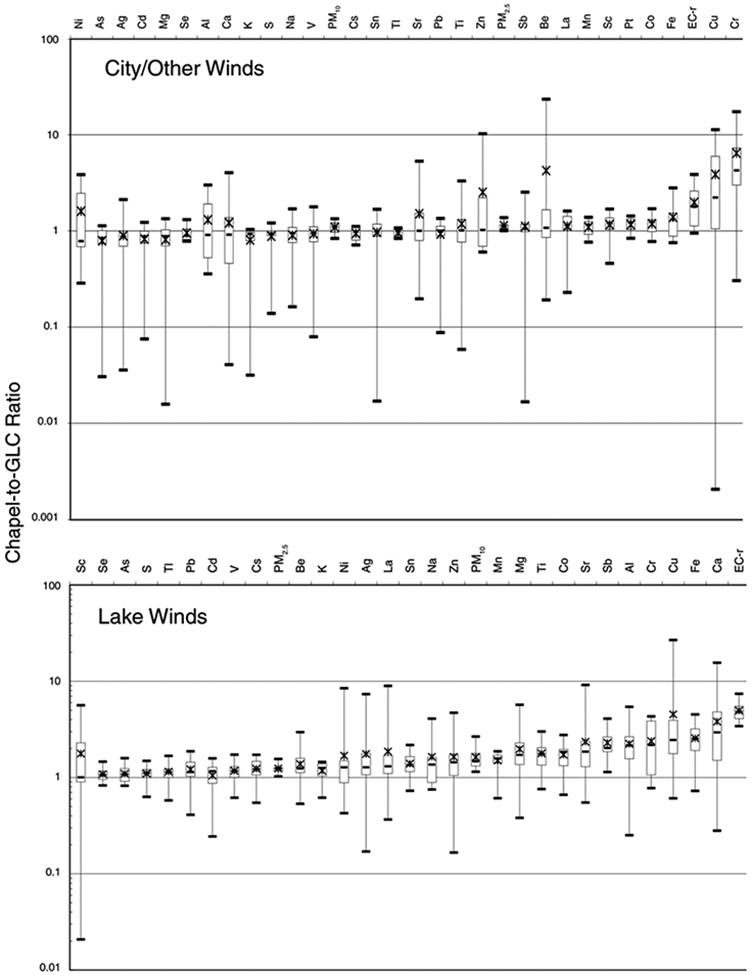
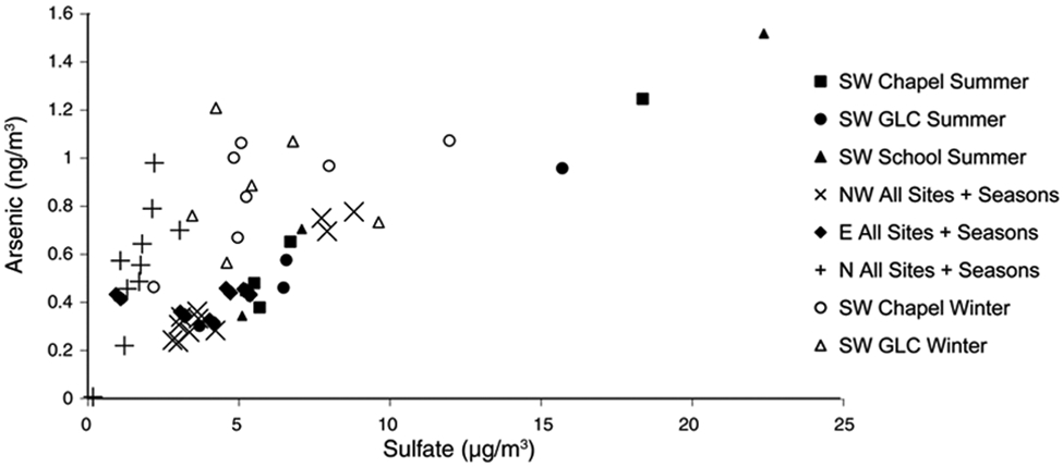
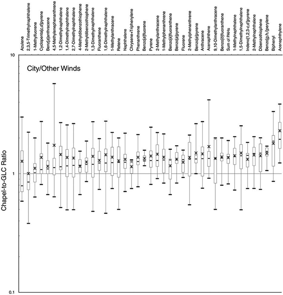
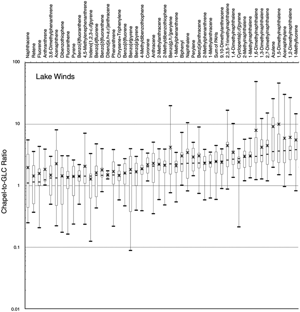
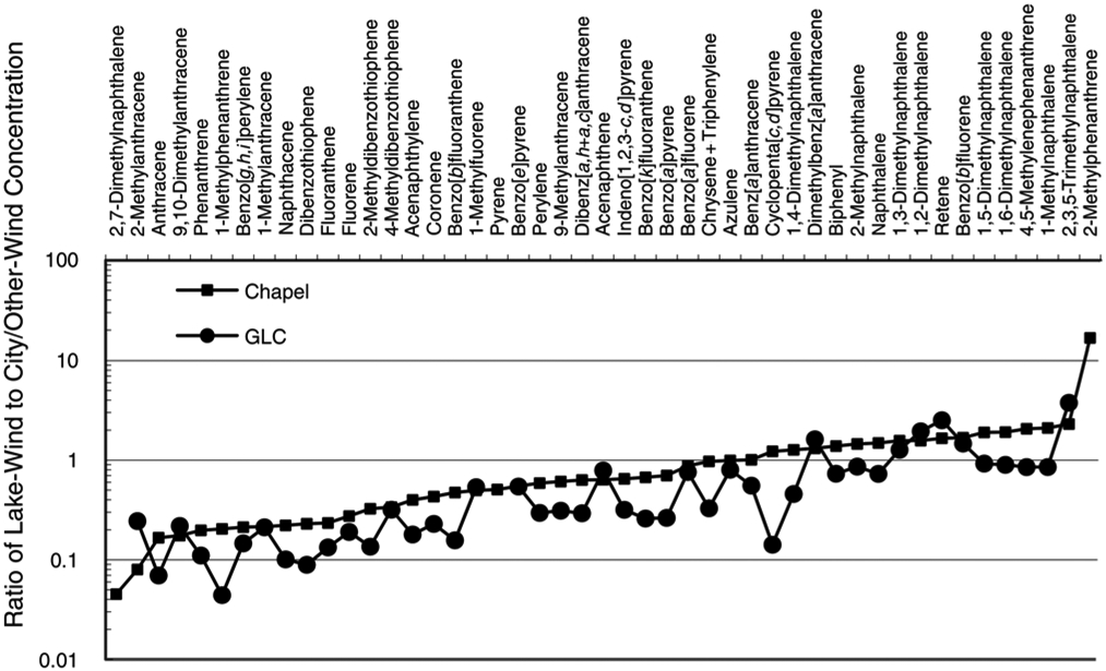
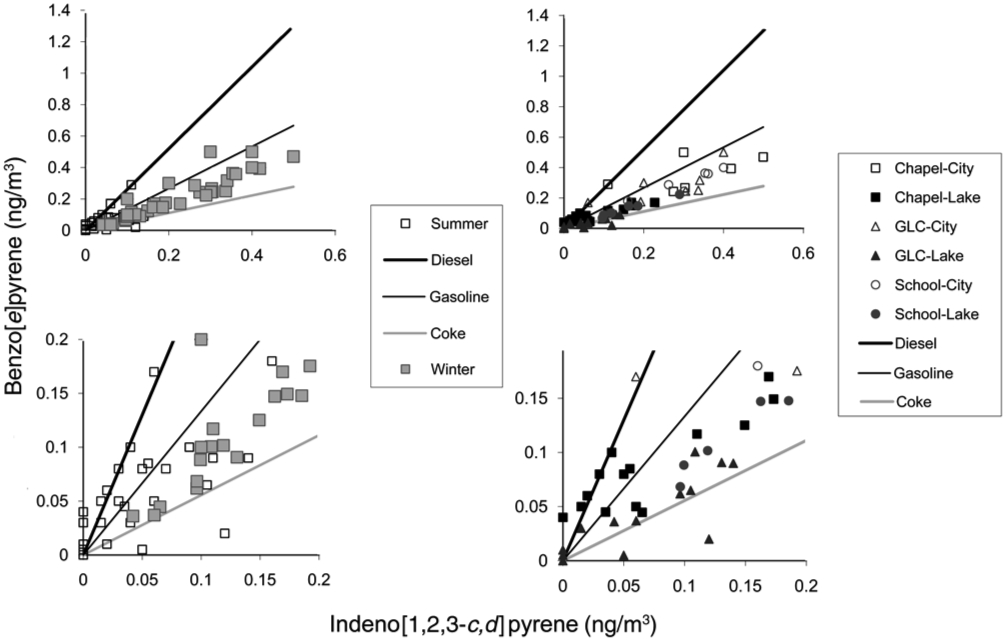
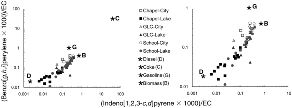
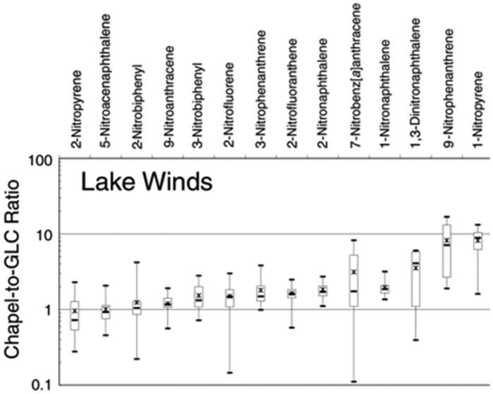
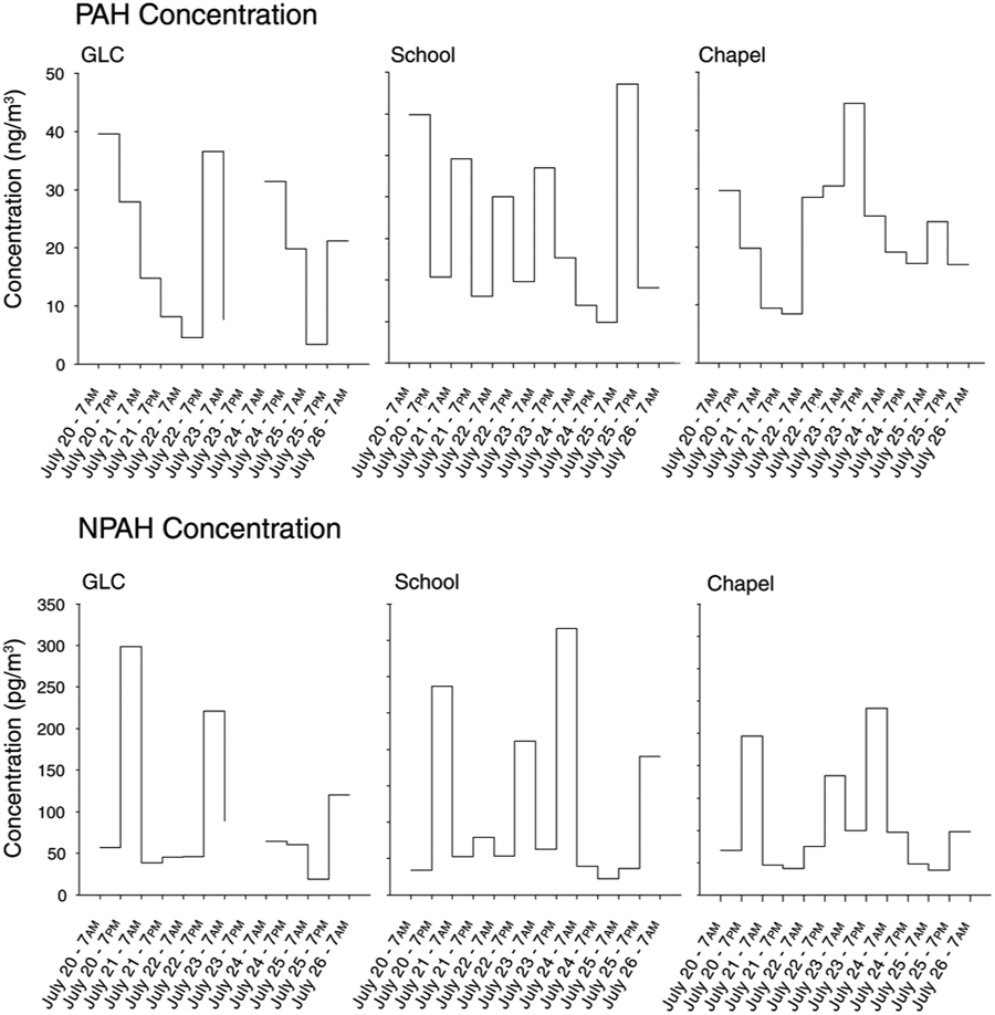
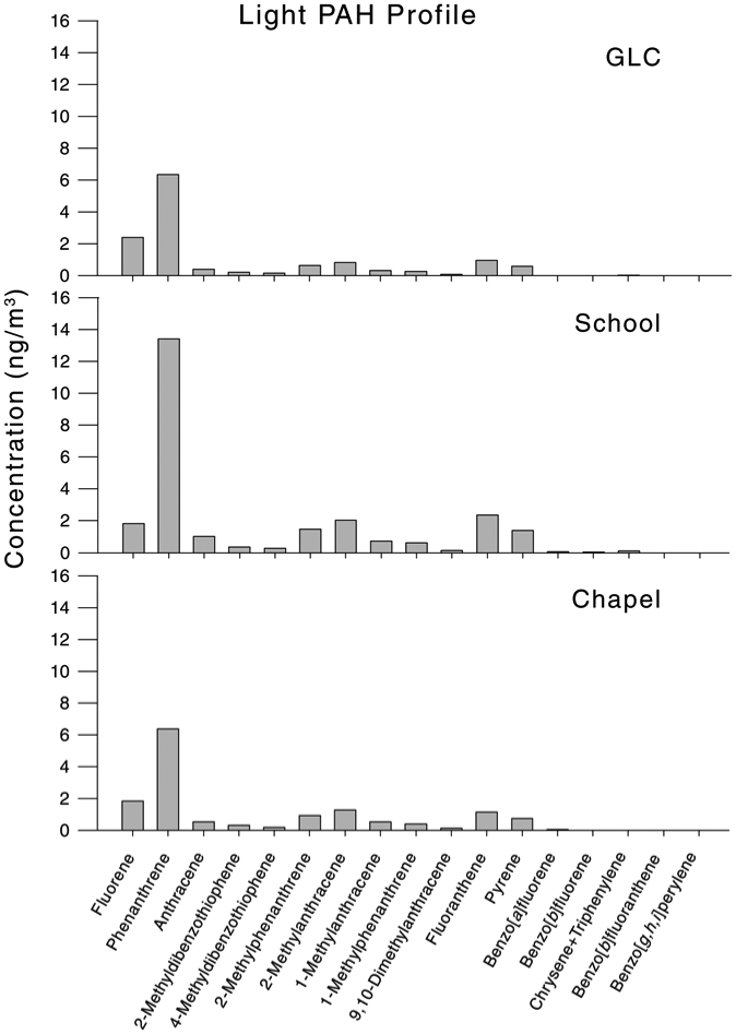
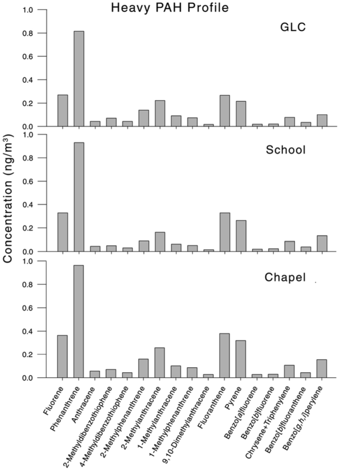
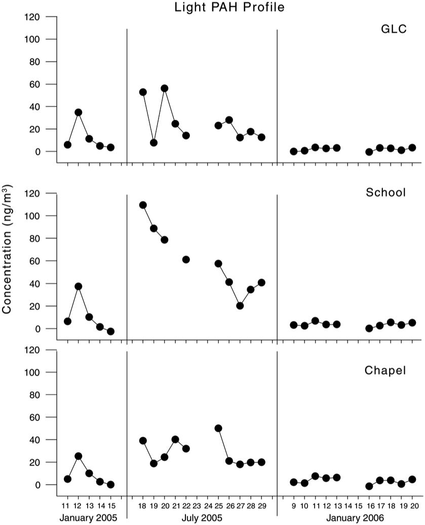
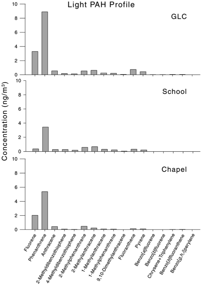
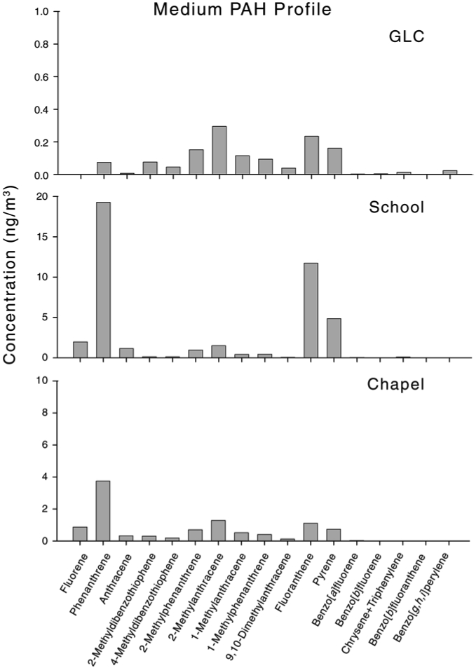
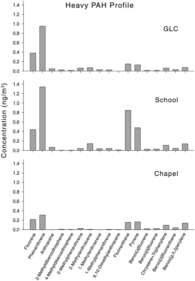
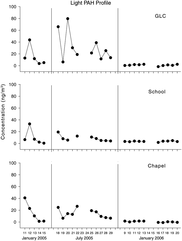
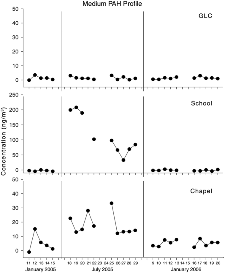
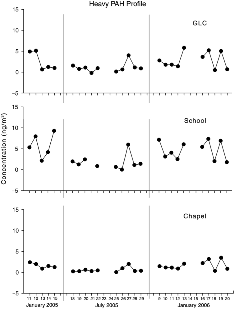
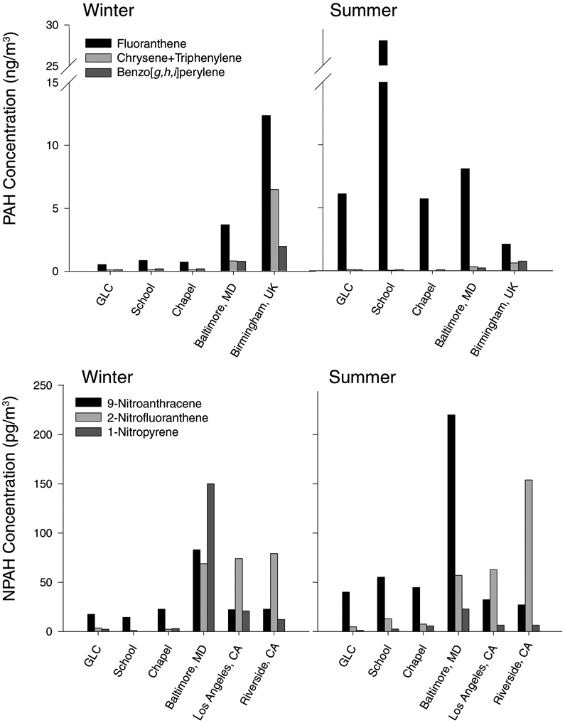
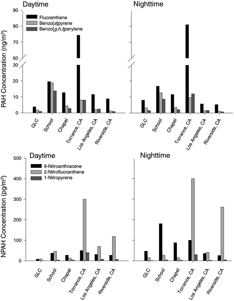
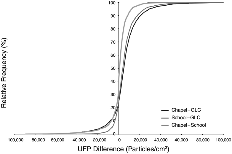
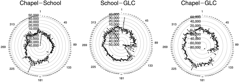
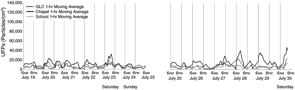
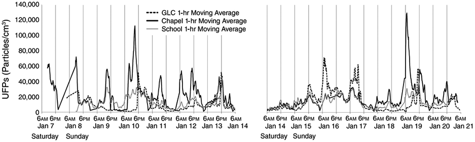
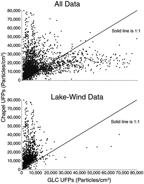
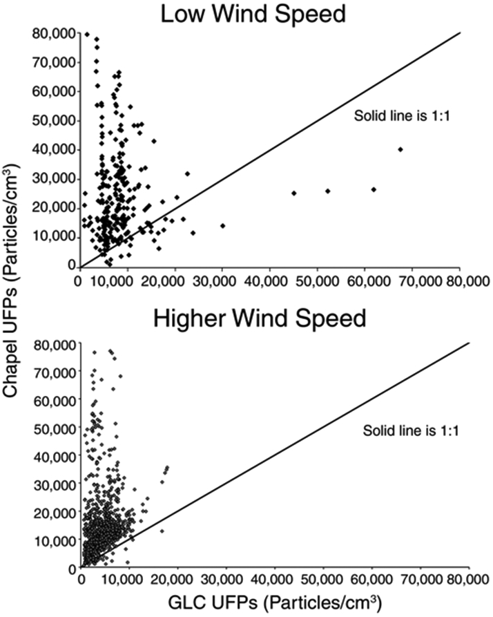
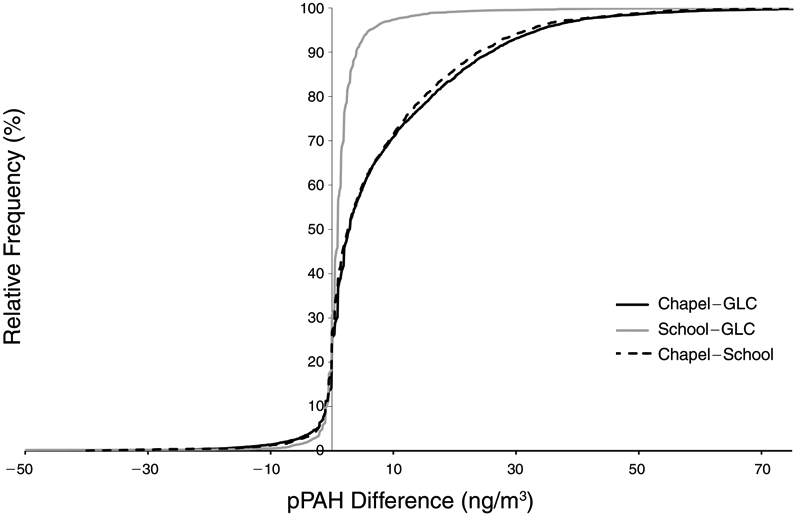
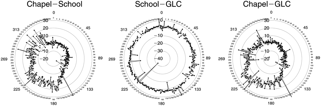
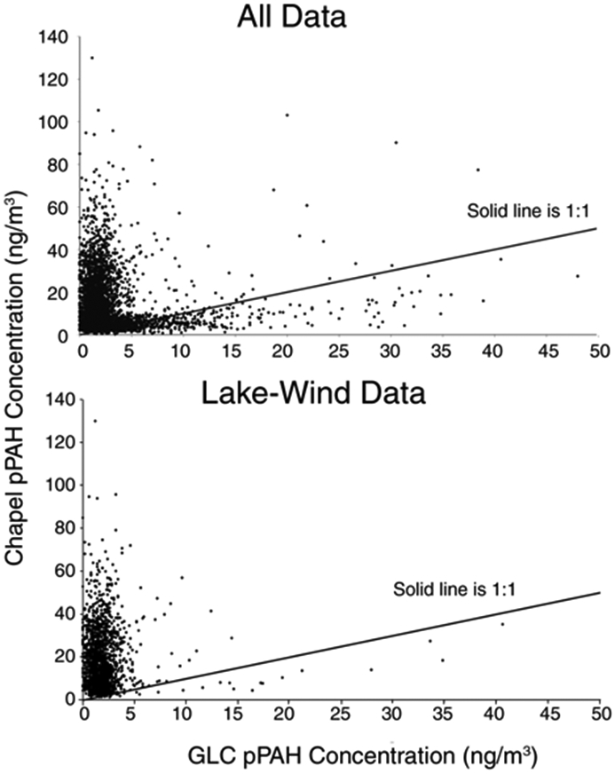
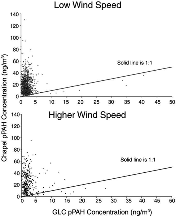
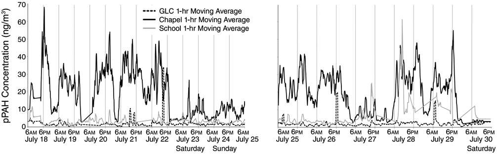
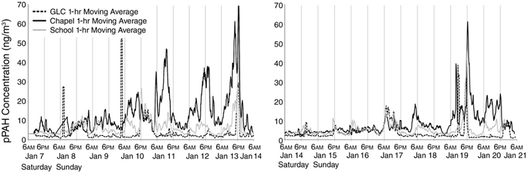
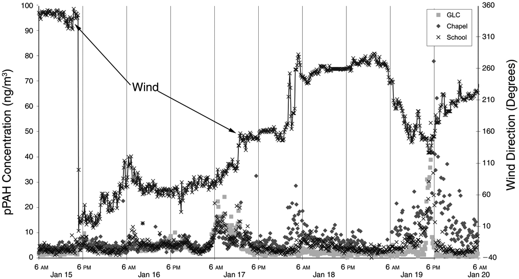
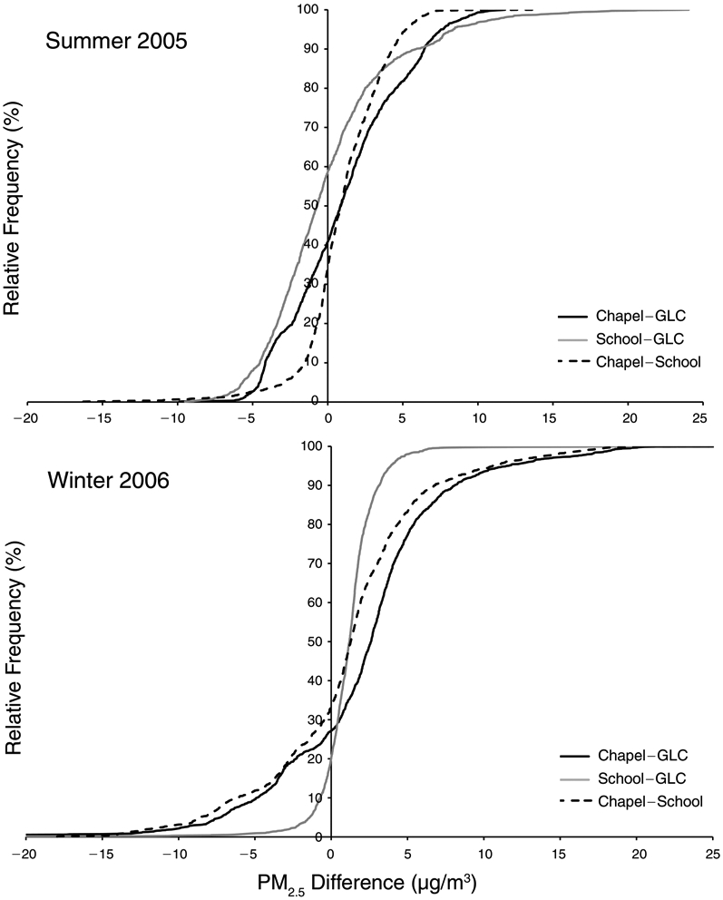
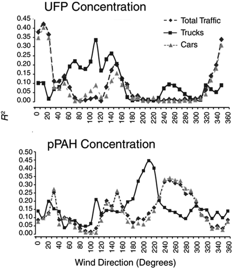
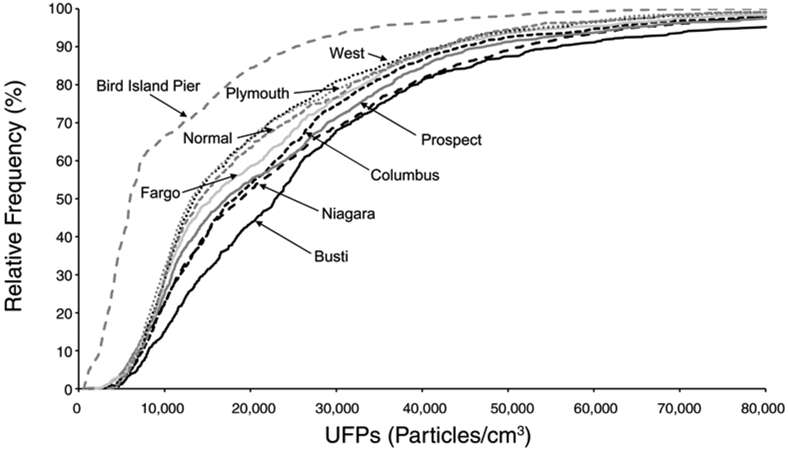
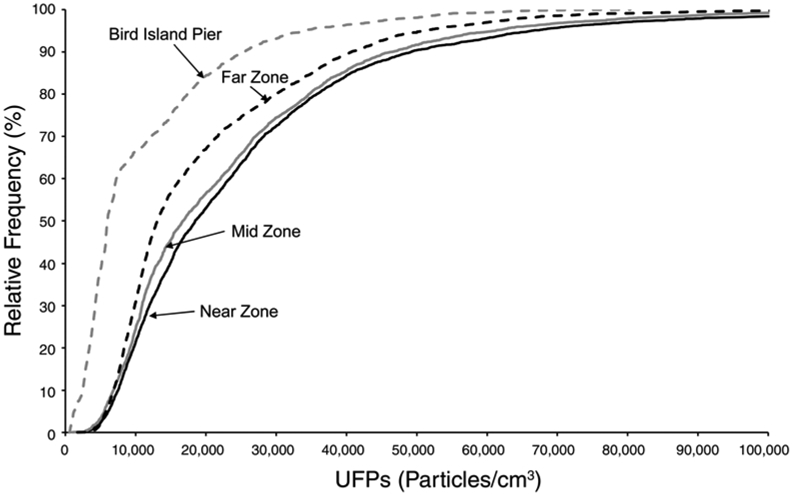
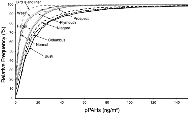
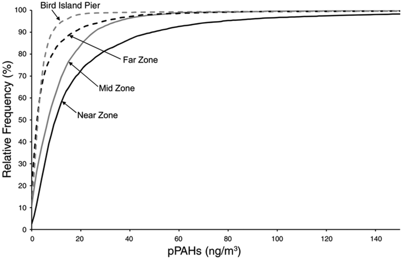
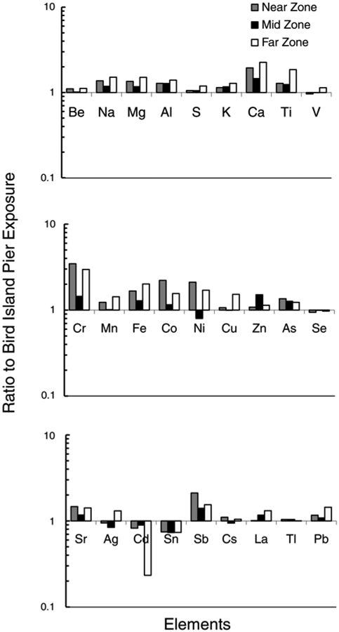
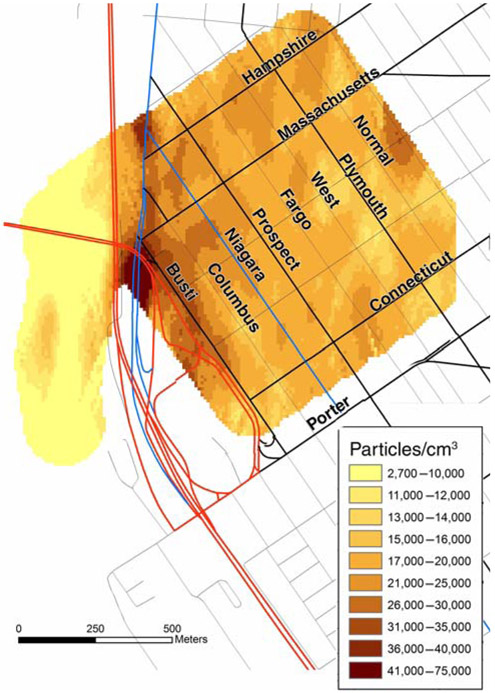
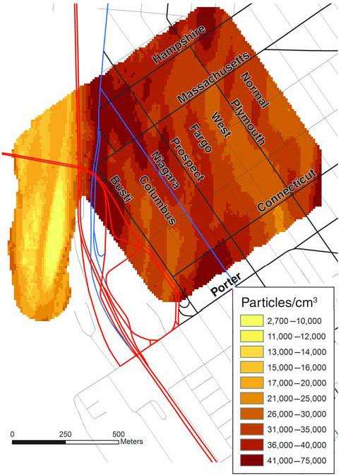
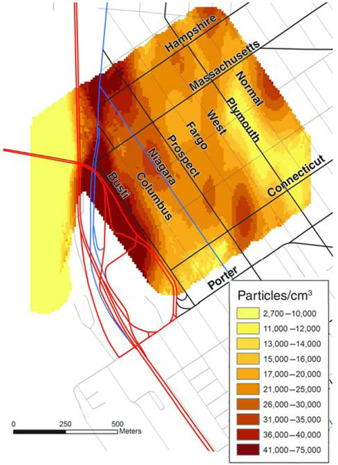
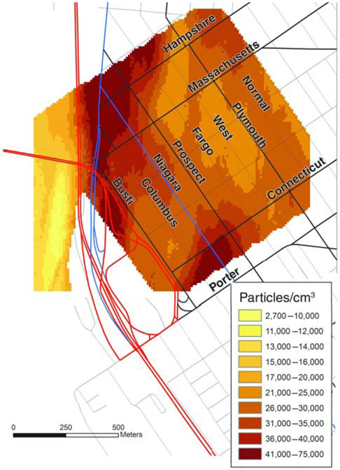
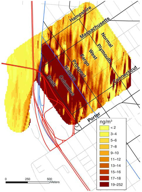
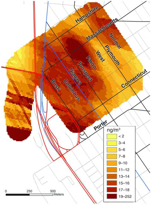
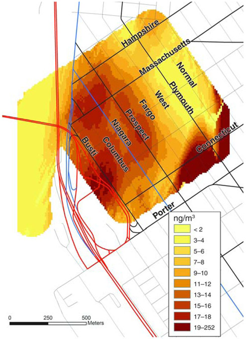
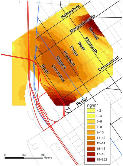
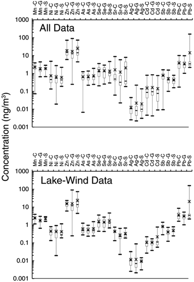
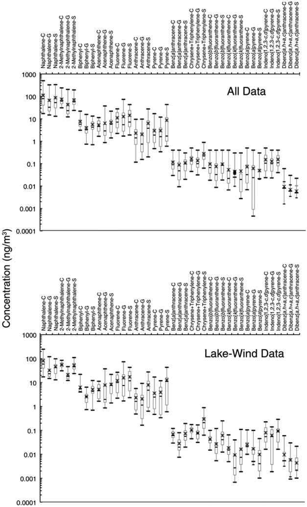
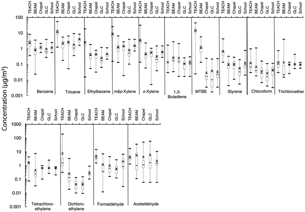
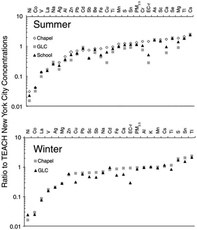
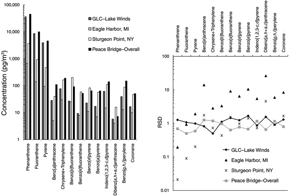
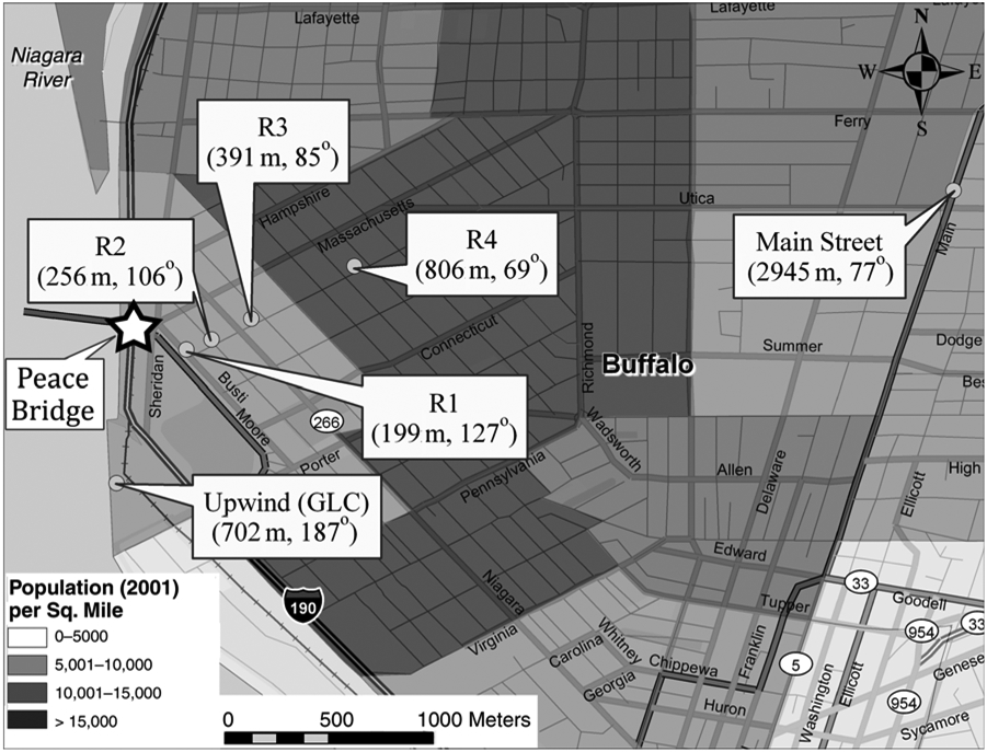
The Peace Bridge in Buffalo, New York, which spans the Niagara River at the east end of Lake Erie, is one of the busiest U.S. border crossings. The Peace Bridge plaza on the U.S. side is a complex of roads, customs inspection areas, passport control areas, and duty-free shops. On average 5000 heavy-duty diesel trucks and 20,000 passenger cars traverse the border daily, making the plaza area a potential "hot spot" for emissions from mobile sources. In a series of winter and summer field campaigns, we measured air pollutants, including many compounds considered by the U.S. Environmental Protection Agency (EPA*) as mobile-source air toxics (MSATs), at three fixed sampling sites: on the shore of Lake Erie, approximately 500 m upwind (under predominant wind conditions) of the Peace Bridge plaza; immediately downwind of (adjacent to) the plaza; and 500 m farther downwind, into the community of west Buffalo. Pollutants sampled were particulate matter (PM) < or = 10 microm (PM10) and < or = 2.5 microm (PM2.5) in aerodynamic diameter, elemental carbon (EC), 28 elements, 25 volatile organic compounds (VOCs) including 3 carbonyls, 52 polycyclic aromatic hydrocarbons (PAHs), and 29 nitrogenated polycyclic aromatic hydrocarbons (NPAHs). Spatial patterns of counts of ultrafine particles (UFPs, particles < 0.1 microm in aerodynamic diameter) and of particle-bound PAH (pPAH) concentrations were assessed by mobile monitoring in the neighborhood adjacent to the Peace Bridge plaza using portable instruments and Global Positioning System (GPS) tracking. The study was designed to assess differences in upwind and downwind concentrations of MSATs, in areas near the Peace Bridge plaza on the U.S. side of the border. The Buffalo Peace Bridge Study featured good access to monitoring locations proximate to the plaza and in the community, which are downwind with the dominant winds from the direction of Lake Erie and southern Ontario. Samples from the lakeside Great Lakes Center (GLC), which is upwind of the plaza with dominant winds, were used to characterize contaminants in regional air masses. On-site meteorologic measurements and hourly truck and car counts were used to assess the role of traffic on UFP counts and pPAH concentrations. The array of parallel and perpendicular residential streets adjacent to the plaza provided a grid on which to plot the spatial patterns of UFP counts and pPAH concentrations to determine the extent to which traffic emissions from the Peace Bridge plaza might extend into the neighboring community. For lake-wind conditions (southwest to northwest) 12-hour integrated daytime samples showed clear evidence that vehicle-related emissions at the Peace Bridge plaza were responsible for elevated downwind concentrations of PM2.5, EC, and benzene, toluene, ethylbenzene, and xylenes (BTEX), as well as 1,3-butadiene and styrene. The chlorinated VOCs and aldehydes were not differentially higher at the downwind site. Several metals (aluminum, calcium, iron, copper, and antimony) were two times higher at the site adjacent to the plaza as they were at the upwind GLC site on lake-wind sampling days. Other metals (beryllium, sodium, magnesium, potassium, titanium, manganese, cobalt, strontium, tin, cesium, and lanthanum) showed significant increases downwind as well. Sulfur, arsenic, selenium, and a few other elements appeared to be markers for regional transport as their upwind and downwind concentrations were correlated, with ratios near unity. Using positive matrix factorization (PMF), we identified the sources for PAHs at the three fixed sampling sites as regional, diesel, general vehicle, and asphalt volatilization. Diesel exhaust at the Peace Bridge plaza accounted for approximately 30% of the PAHs. The NPAH sources were identified as nitrate (NO3) radical reactions, diesel, and mixed sources. Diesel exhaust at the Peace Bridge plaza accounted for 18% of the NPAHs. Further evidence for the impact of the Peace Bridge plaza on local air quality was found when the differences in 10-minute average UFP counts and pPAH concentrations were calculated between pairs of sites and displayed by wind direction. With winds from approximately 160 degrees through 220 degrees, UFP counts adjacent to the plaza were 10,000 to 20,000 particles/cm3 higher than those upwind of the plaza. A similar pattern was displayed for pPAH concentrations adjacent to the plaza, which were between 10 and 20 ng/m3 higher than those at the upwind GLC site. Regression models showed better correlation with traffic variables for pPAHs than for UFPs. For pPAHs, truck counts and car counts had significant positive correlations, with similar magnitudes for the effects of trucks and cars, despite lower truck counts. Examining all traffic variables, including traffic counts and counts divided by wind speed, the multivariate regression analysis had an adjusted coefficient of determination (R2) of 0.34 for pPAHs, with all terms significant at P < 0.002. Study staff members traversed established routes in the neighborhood while carrying instruments to record continuous UFP and pPAH values. They also carried a GPS, which was used to provide location-specific time-stamped data. Analyses using a geographic information system (GIS) demonstrated that emissions at the Peace Bridge plaza, at times, affected ambient air quality over several blocks (a few hundred meters). Under lake-wind conditions, overall spatial patterns in UFP and pPAH levels were similar for summer and winter and for morning and afternoon sampling sessions. The Buffalo Peace Bridge Study demonstrated that a concentration of motor vehicles resulted in elevated levels of mobile-source-related emissions downwind, to distances of 300 m to 600 m. The study provides a unique data set to assess interrelationships among MSATs and to ascertain the impact of heavy-duty diesel vehicles on air quality.


Figures

Figure A.1.
Figure A.1.. Comparison of the mean concentration of high-molecular-weight PAHs (ng/m3) for the GLC and School sites overall against the corresponding mean PAS PAH reading.
By averaging over all of the sampling sessions, the day-to-day variation in the ratio between compounds in the gas phase and compounds in the particle can be smoothed out.
Figure A.2.
Figure A.2.. Comparison of high-molecular-weight PAH concentrations (ng/m3) in the integrated 12-hour samples and the mean PAS samples for the corresponding time periods (winter and summer sampling sessions) for all samples where air mass trajectories were primarily over water.
Figure A.3.
Figure A.3.. Comparison of wind speeds (mph) between the Buffalo Airport and the GLC Davis Weather Station for summer 2005 sampling session.
Figure A.4.
Figure A.4.. Histogram of wind speed differences (mph) between the Buffalo Airport and the GLC site for summer 2005 sampling session.
Figure A.5.
Figure A.5.. Comparison of wind direction (degrees) between the Buffalo Airport and the GLC Davis Weather Station for summer 2005 sampling session (seven pairs of measurements with one value greater than 0 and the other less than 360 have been removed).
Figure A.6.
Figure A.6.. Histogram of differences in wind speed directions (degrees) between the Buffalo Airport and the GLC Davis Weather Station for summer 2005 sampling session.
Figure 1.
Figure 1.. The study area comprised the Peace Bridge plaza and the three fixed sampling sites (GLC, Chapel, and School), as well as Bird Island Pier and the neighborhood of west Buffalo (boxed), where routes for mobile monitoring were located.
Figure 2.
Figure 2.. Wind rose showing 1992 annual average wind speed and direction for Buffalo, from the Buffalo Niagara International Airport (15 km east-northeast of the Peace Bridge plaza).
Source: Buffalo Airport Scram Surface Met Data 1992 (available from www.webmet.com; accessed October 27, 2010).
Figure 3.
Figure 3.. Hourly counts of total traffic and truck traffic on the Peace Bridge (June 20–26, 2004), showing a cyclic pattern with lows late at night and peaks during the day.
Note different scales for y axes.
Figure 4.
Figure 4.. Mobile monitoring routes.
Data points represent GPS points recorded by devices that field staff carried in their backpacks as they walked the routes.
Figure 5.
Figure 5.. Cumulative distributions of hourly counts of total traffic, trucks, and cars on the Peace Bridge during sampling sessions, compared with seasonal and annual data.
Figure 6.
Figure 6.. Peace Bridge vehicle counts per hour, winter 2005 sampling session.
Figure 7.
Figure 7.. Peace Bridge vehicle counts per hour, summer 2005 sampling session.
Figure 8.
Figure 8.. Peace Bridge vehicle counts per hour, winter 2006 sampling session.
Figure 9.
Figure 9.. Backward air mass trajectories and wind directions for the first week of the winter 2005 sampling session.
Figure 10.
Figure 10.. Backward air mass trajectories and wind directions for the second week of the winter 2005 sampling session.
Figure 11.
Figure 11.. Backward air mass trajectories and wind directions for the first week of the summer 2005 sampling session.
Figure 12.
Figure 12.. Backward air mass trajectories and wind directions for the second week of the summer 2005 sampling session.
Figure 13.
Figure 13.. Backward air mass trajectories and wind directions for the first week of the winter 2006 sampling session.
Figure 14.
Figure 14.. Backward air mass trajectories and wind directions for the second week of the winter 2006 sampling session.
Figure 15.
Figure 15.. Chapel-to-GLC ratios for the sum of PAH measurements and EC-r measurements: 12-hour weekday integrated samples (N = 22).
Figure 16.
Figure 16.. Box and whisker plots of Chapel-to-GLC ratios for VOC, PM2.5, and EC-r values on city-wind days (N = 7 pairs) and lake-wind days (N = 14 pairs).
Minimum, bottom whisker; 25th percentile, bottom of the box; median, center line in the box; mean, “x”; 75th percentile, top of the box; and maximum, top whisker. For city/other-wind days all compounds, except chloroform, had at least 5 pairs of samples above LOD (chloroform is not shown). For lake-wind days formaldehyde, 1,4-dichlorobenzene, acetone, and trichloroethene had 5 of 14 sample pairs above LOD. Compounds are ranked by the median ratio.
Figure 17.
Figure 17.. University of California–Davis average acrolein levels obtained at the Chapel site on July 25, 2004.
Figure 18.
Figure 18.. Box and whisker plots of Chapel-to-GLC ratios for 28 elements, PM10, PM2.5, and EC-r on city/other-wind days (N = 8 pairs) and lake-wind days (N = 15 pairs).
Minimum, bottom whisker; 25th percentile, bottom of the box; median, center line in the box; mean, “x”; 75th percentile, top of the box; and maximum, top whisker. Compounds are rank ordered by median ratio.
Figure 19.
Figure 19.. Edge plot of ratios of arsenic to sulfate concentrations with air mass trajectories from different directions.
Data for the north, east, and northwest trajectories are for all sites and seasons; data for the southwest trajectory are presented by site and season.
Figure 20.
Figure 20.. Box and whisker plots of Chapel-to-GLC ratios for PAHs and sum of PAHs (N = 8 pairs) with city/other winds.
Minimum, bottom whisker; 25th percentile, bottom of the box; median, center line in the box; mean, “x”; 75th percentile, top of the box; and maximum, top whisker. All compounds have at least five pairs of samples above the LOD. 3-Methylchloanthrene, 9-methylanthracene, 3,6-dimethylphenanthrene, benzo[b]fluorene, naphthacene, 4-methylchrysene, dimethylbenz[a]anthracene, perylene, dibenz[a,h+a,c]anthracene, anthranthrene, and coronene are not shown. Compounds are ordered by the median ratio.
Figure 21.
Figure 21.. Box and whisker plots of Chapel-to-GLC ratios for PAHs and sum of PAHs (N = 14 pairs) with lake winds.
Minimum, bottom whisker; 25th percentile, bottom of the box; median, center line in the box; mean, “x”; 75th percentile, top of the box; and maximum, top whisker. All compounds have at least five pairs of samples above the LOD. 3-Methylchloanthrene, 9-methylanthracene, 3,6-dimethylphenanthrene, benzo[b]fluorene, naphthacene, 4-methylchrysene, dimethylbenz[a]anthracene, and anthranthrene are not shown. Compounds are ordered by the median ratios.
Figure 22.
Figure 22.. Ratios of median lake-wind PAH concentrations to median city/other-wind PAH concentrations measured at the Chapel and GLC sites.
Compounds are rank ordered by Chapel site values.
Figure 23.
Figure 23.. Edge plots of benzo[e]pyrene and indeno[1,2,3-c,d]pyrene by season (summer and winter), and by sampling site paired with wind direction.
The plots at the bottom are magnifications of the low values in the top plots.
Figure 24.
Figure 24.. Ratio-to-ratio plots of (benzo[g,h,i]perylene × 1000)/EC and (indeno[1,2,3-c,d]pyrene × 1000)/EC.
The plot on the right is a magnification of the low values in the plot on the left.
Figure 25.
Figure 25.. Box and whisker plots of Chapel-to-GLC ratios for NPAHs (N = 10 pairs) with lake winds.
Minimum, bottom whisker; 25th percentile, bottom of the box; median, center line in the box; mean, “x”; 75th percentile, top of the box; and maximum, top whisker.
Figure 26.
Figure 26.. Diurnal pattern of total PAH and NPAH concentrations at the GLC, School, and Chapel sites during July 2005, from data obtained using Graseby Andersen high-volume samplers.
Figure 27.
Figure 27.. Light PAH profile and heavy PAH profile based on lighter-molecular-weight and heavier-molecular-weight PAHs, resolved by two-source PMF analysis of seasonal data (winter 2005, summer 2005, and winter 2006 samples).
Figure 27.
Figure 27.. Light PAH profile and heavy PAH profile based on lighter-molecular-weight and heavier-molecular-weight PAHs, resolved by two-source PMF analysis of seasonal data (winter 2005, summer 2005, and winter 2006 samples).
Figure 28.
Figure 28.. Temporal patterns of light PAH profile and heavy PAH profile concentrations resolved by two-source PMF analysis.
Figure 28.
Figure 28.. Temporal patterns of light PAH profile and heavy PAH profile concentrations resolved by two-source PMF analysis.
Figure 29.
Figure 29.. Light, medium, and heavy PAH profiles resolved by three-source PMF analysis of PAH data.
Figure 29.
Figure 29.. Light, medium, and heavy PAH profiles resolved by three-source PMF analysis of PAH data.
Figure 29.
Figure 29.. Light, medium, and heavy PAH profiles resolved by three-source PMF analysis of PAH data.
Figure 30.
Figure 30.. Temporal pattern of the light, medium, and heavy PAH profiles in winter 2005, summer 2005, and winter 2006, resolved by three-source PMF analysis.
Figure 30.
Figure 30.. Temporal pattern of the light, medium, and heavy PAH profiles in winter 2005, summer 2005, and winter 2006, resolved by three-source PMF analysis.
Figure 30.
Figure 30.. Temporal pattern of the light, medium, and heavy PAH profiles in winter 2005, summer 2005, and winter 2006, resolved by three-source PMF analysis.
Figure 31.
Figure 31.. Comparison of selected PAHs and NPAHs measured at the three sampling sites in Buffalo (GLC, School, Chapel) during the summer and winter with those reported in other locations: Buffalo, means of 15 samples measured in January 2005 and 2006 and 10 samples (9 for School site) in July 2005 (this study); Baltimore, geometric means of 69 samples measured in summer 2002 and winter 2003 (Crimmins 2006); Birmingham, means of 55 samples collected in February and August 1992 (Harrison et al. 1996); Los Angeles and Riverside, means of four 5-day samples collected at different time intervals in August 2002 and four collected in January 2003 (Reisen and Arey 2005).
Figure 32.
Figure 32.. Comparison of selected PAHs and NPAHs measured at the three sampling sites in Buffalo (GLC, School, Chapel) during the daytime and nighttime with those reported in three California locations: Buffalo, means of 4 samples measured during the daytime (7:00 am to 7:00 pm) in July 2004 and during the nighttime (7:00 pm to 7:00 am) in July 2005 (this study); Torrance, means of 6 filter samples measured during the daytime (6:00 am to 6:00 pm) and the nighttime (6:00 pm to 6:00 am) in February 1986 (Arey et al. 1987); Los Angeles and Riverside, means of 5-day sampling at 4 time intervals during the daytime (7:00 am to 6:30 pm) and nighttime (7:00 pm to 6:30 am) in August 2002 (Reisen and Arey 2005).
Figure 33.
Figure 33.. Cumulative frequency distributions of the differences in 10-minute average UFP counts between fixed sampling sites.
Figure 34.
Figure 34.. Radial plots of differences in UFP concentrations (particles/cm3) between the Chapel and School, School and GLC, and Chapel and GLC sites, by wind direction.
From a data set of average wind direction and concentration data for 10-minute periods during winter 2005, summer 2005, and winter 2006 sampling sessions, the average of the 10-minute average differences in concentration was calculated for each wind direction degree.
Figure 35.
Figure 35.. UFP counts (hourly moving average) at the three sampling sites during the summer 2005 sampling session.
Figure 36.
Figure 36.. UFP counts (hourly moving average) at the three sampling sites during the winter 2006 sampling session.
Figure 37.
Figure 37.. UFP counts at the Chapel site versus those at the GLC site: all data and data obtained under lake-wind conditions (wind direction, 180°–280°).
Figure 38.
Figure 38.. UFP counts at the Chapel site versus those at the GLC site obtained during lake winds of low speed (≤ 3.1 m/sec) and higher speed (> 3.1 m/sec).
Figure 39.
Figure 39.. Cumulative frequency distributions of the differences in pPAH 10-minute average concentrations between sampling sites.
Figure 40.
Figure 40.. Radial plots of differences between pPAH concentrations (ng/m3) at the Chapel and School, School and GLC, and Chapel and GLC sites, by wind direction.
From a data set of 10-minute average wind directions and pPAH concentrations for winter 2005, summer 2005, and winter 2006 sampling sessions, the average difference of the 10-minute average concentrations was calculated for each wind direction degree.
Figure 41.
Figure 41.. Scatter plot of all pPAH concentrations from the summer 2005 and winter 2006 sampling sessions for the Chapel site versus the GLC site; and scatter plot of concentrations measured under lake-wind conditions (wind direction, 180°–280°).
Figure 42.
Figure 42.. Scatter plot of pPAH concentrations from the summer 2005 and winter 2006 sampling sessions for the Chapel site versus the GLC site measured during lake winds of low speed (≤ 3.1 m/sec); and scatter plot of concentrations measured under lake winds of higher speed (> 3.1 m/sec).
Figure 43.
Figure 43.. One-hour moving average pPAH concentrations during the summer 2005 sampling session for the three sampling sites.
Figure 44.
Figure 44.. One-hour moving average pPAH concentrations during the winter 2006 sampling session for the three sampling sites.
Figure 45.
Figure 45.. Ten-minute average pPAH concentrations and wind directions for selected days in winter 2006.
Figure 46.
Figure 46.. Cumulative frequency distributions of the differences in 10-minute average PM2.5 concentrations between sampling sites, for the summer 2005 and winter 2006 sampling sessions.
Figure 47.
Figure 47.. Coefficient of determination (R2) for the Chapel site UFP concentrations and pPAH concentrations versus car, truck, and total traffic counts reported by the Peace Bridge Authority.
R2 was computed between the pollutant concentrations for each average wind direction stratified by wind-angle increment of 10° ± 30° and the hourly traffic counts categorized by vehicle types.
Figure 48.
Figure 48.. Cumulative frequency distribution of 1-minute UFP data collected during summer 2005 and winter 2006 mobile monitoring campaigns, classified by street.
Figure 49.
Figure 49.. Cumulative frequency distribution of 1-minute UFP data collected during summer 2005 and winter 2006 mobile monitoring campaigns, classified by neighborhood zone.
Figure 50.
Figure 50.. Cumulative frequency distribution of 1-minute pPAH data collected during summer 2005 and winter 2006 mobile monitoring campaigns, classified by street.
Figure 51.
Figure 51.. Cumulative frequency distribution of 1-minute pPAH data collected during summer 2005 and winter 2006 mobile monitoring campaigns, classified by neighborhood zone.
Figure 52.
Figure 52.. Ratio of exposures to elements on the mobile monitoring routes in the near, mid, and far zones to values on the Bird Island Pier route (background).
Values are the means of data from 4 samplers worn by staff in summer 2005 while walking the routes. Each sample is a composite of several route-days.
Figure 53.
Figure 53.. Spatial pattern of combined summer and winter UFP measurements (N = 10,808) made under lake-wind conditions in west Buffalo using P-Trak.
Figure 54.
Figure 54.. Spatial pattern of combined summer and winter UFP measurements (N = 3980) made under city-wind conditions in west Buffalo using P-Trak.
Figure 55.
Figure 55.. Spatial pattern of UFP measurements (N = 2478) made on winter mornings under lake-wind conditions in west Buffalo using P-Trak.
Figure 56.
Figure 56.. Spatial pattern of UFP measurements (N = 2373) made on winter afternoons under lake-wind conditions in west Buffalo using P-Trak.
Figure 57.
Figure 57.. Spatial pattern of UFP measurements (N = 2331) made on winter mornings under city-wind conditions in west Buffalo using P-Trak.
Figure 58.
Figure 58.. Spatial pattern of combined summer and winter pPAH measurements (N = 12,821) made under lake-wind conditions in west Buffalo using a PAS.
Figure 59.
Figure 59.. Spatial pattern of combined summer and winter pPAH measurements (N = 4637) made under city-wind conditions in west Buffalo using a PAS.
Figure 60.
Figure 60.. Spatial pattern of pPAH measurements (N = 2978) made on winter mornings under lake-wind conditions in west Buffalo using a PAS.
Figure 61.
Figure 61.. Spatial pattern of pPAH measurements (N = 2522) made on winter mornings under city-wind conditions in west Buffalo using a PAS.
Figure 62.
Figure 62.. Box and whisker plots of concentrations of MSAT elements at the Chapel (C), GLC (G), and School (S) sites for all data (N = 24) and for data obtained on lake-wind days (N = 15).
Minimum, bottom whisker; 25th percentile, bottom of the box; median, center line in the box; mean, “x”; 75th percentile, top of the box; and maximum, top whisker.
Figure 63.
Figure 63.. Box and whisker plots of concentrations of MSAT PAHs at the Chapel (C), GLC (G), and School (S) sites for all data (N = 24) and for data obtained on lake-wind days (N = 14).
Minimum, bottom whisker; 25th percentile, bottom of the box; median, center line in the box; mean, “x”; 75th percentile, top of the box; and maximum, top whisker.
Figure 64.
Figure 64.. Box and whisker plots of concentrations of MSAT VOCs, BTEX, and BTEX plus compounds, chlorinated compounds, and carbonyls at the Chapel (C), GLC (G), and School (S) sites for all data (N = 24) and for data obtained on lake-wind days (N = 14).
Minimum, bottom whisker; 25th percentile, bottom of the box; median, center line in the box; mean, “x”; 75th percentile, top of the box; and maximum, top whisker.
Figure 65.
Figure 65.. Box and whisker plots of VOC concentrations at the Chapel, GLC, and School sites in this study and outdoor concentrations from the TEACH study in Los Angeles and the BEAM study in Boston.
Minimum, bottom whisker; 25th percentile, bottom of the box; median, center line in the box; mean, “x”; 75th percentile, top of the box; and maximum, top whisker.
Figure 66.
Figure 66.. Seasonal comparison of median element concentrations in Buffalo (this study) and in New York City (TEACH study, in which N = 36 for both winter and summer).
Figure 67.
Figure 67.. Left: Mean PAH concentrations at the GLC site under lake-wind conditions (N = 14), in the Peace Bridge Study samples overall (N = 67), and in samples taken by the Integrated Atmospheric Deposition Network at Eagle Harbor and Sturgeon Point (N = 100; analyte detection, 42%–100%). Right: Reported relative standard deviations of measurements (SD/mean) in these sample sets.
Eagle Harbor is on the shore of Lake Superior and represents regional background levels; data were from November 1990 through December 1997. Sturgeon Point is on the shore of Lake Erie, in the Buffalo area; data were from December 1991 through December 1997. (Data are from Cortes et al. 2000.)
Figure 68.
Figure 68.. Map showing the location and sampling sites used in the Clarkson University study.
The reported distances are measured to an arbitrary center point of the Peace Bridge, marked with a star on the map. The wind direction was generally southwesterly over the sampling period. Adapted with permission from Ogulei et al. 2007, and from the Air and Waste Management Association.
Figure 69.
Figure 69.. Average number concentrations (particles/cm3) measured at the six Clarkson University sampling sites on June 24, 2004, when winds consistently blew from the southwest.
Main Street measurements were made on June 23, 2004. For completeness the entire particle size range measured is shown (6–500 nm). Adapted with permission from Ogulei et al. 2007, and from the Air and Waste Management Association.

Similar articles

Cited by

References

    1. Abu-Allaban M, Gillies JA, Gertler AW, Clayton R, Proffitt D. 2003. Tailpipe, resuspended road dust, and brake-wear emission factors from on-road vehicles. Atmos Environ 37:5283–5293.
    1. Ahlbom J, Duns U. 1994. Nya hjulspår – en produkstudie av gummidäck. Rapport från kemikalienspektionen i samarbete med länsstyrelsen (Gothenburg).
    1. Antweiler RC, Taylor HE. 2008. Evaluation of statistical treatments of left-censored environmental data using coincident uncensored datasets. 1: Summary statistics. Environ Sci Technol 42:3732–3738. - PubMed
    1. Arey J. 1998. Atmospheric reactions of PAHs including formation of nitroarenes. In: Vol 3, The Handbook of Environmental Chemistry (Neilson AH, ed). Springer, Berlin, Germany.
    1. Arey J, Zielinska B, Atkinson R, Winer AM. 1987. Polycyclic aromatic hydrocarbon and nitroarene concentrations in ambient air during a wintertime high NOx episode in the Los Angeles basin. Atmos Environ 21:1437–1444.

Publication types