. 2011;6(9):e24523.
doi: 10.1371/journal.pone.0024523. Epub 2011 Sep 9.

Coarse-to-fine changes of receptive fields in lateral geniculate nucleus have a transient and a sustained component that depend on distinct mechanisms

Affiliations

Coarse-to-fine changes of receptive fields in lateral geniculate nucleus have a transient and a sustained component that depend on distinct mechanisms

Gaute T Einevoll et al. PLoS One. 2011.

Abstract

Visual processing in the brain seems to provide fast but coarse information before information about fine details. Such dynamics occur also in single neurons at several levels of the visual system. In the dorsal lateral geniculate nucleus (LGN), neurons have a receptive field (RF) with antagonistic center-surround organization, and temporal changes in center-surround organization are generally assumed to be due to a time-lag of the surround activity relative to center activity. Spatial resolution may be measured as the inverse of center size, and in LGN neurons RF-center width changes during static stimulation with durations in the range of normal fixation periods (250-500 ms) between saccadic eye-movements. The RF-center is initially large, but rapidly shrinks during the first ~100 ms to a rather sustained size. We studied such dynamics in anesthetized cats during presentation (250 ms) of static spots centered on the RF with main focus on the transition from the first transient and highly dynamic component to the second more sustained component. The results suggest that the two components depend on different neuronal mechanisms that operate in parallel and with partial temporal overlap rather than on a continuously changing center-surround balance. Results from mathematical modeling further supported this conclusion. We found that existing models for the spatiotemporal RF of LGN neurons failed to account for our experimental results. The modeling demonstrated that a new model, in which the response is given by a sum of an early transient component and a partially overlapping sustained component, adequately accounts for our experimental data.


Conflict of interest statement

Competing Interests: The authors have declared that no competing interests exist.

Figures

Figure 1
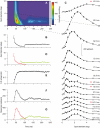
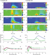
Figure 1. RF dynamically changes during brief stimulus presentation.
Data from an on-center Y-neuron. A, Colormap image of response (z-axis) to a series of spots (n = 25) of different diameters (y-axis) at different time after spot onset (x-axis). Spots were centered on the RF. B, Center-width as function of time after spot onset. Center-width was determined by spot diameter giving maximal response. The RF-center shrank from initially 8 deg to a minimum of 0.5 deg and then increased to a stable width of 2 deg at ∼100 ms. C: Spot width tuning curves for a selected number of time-slices. Notice the truncated x-axis. The time-slice for the spatial summation curve at 52.5 ms is marked by the vertical dashed line in (A), and the first and last data point in this curve are marked by white crosses in (A). Notice the shoulder or bimodal appearance of the curves in the range of 72.5 and 107.5 ms. Single (Eq. 4) and double (Eq. 5) DOG-functions were fitted to the data. Continuous curves show the best-fitting 2-DOG function (linearly interpolated between the spot sizes corresponding to experimental data points). Cases in which the 2-DOG gave statistically better fit than the best-fitting single DOG are marked with asterisk. D, Replot of data in (B) where center width of the transient (red curve) and sustained component (green curve) are separated based on the estimated start of the sustained component, and the end of the first component. E, Development of center-surround antagonism. Notice that 100% antagonism was reached within the first 70 ms. F, Development of the firing rate to the spot that just filled the RF-center. G, Data from (F) separated for the transient (red) and sustained (green) components. Error bars are ±SE. Number of presentations of each spot, 200.
Figure 2
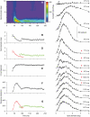
Figure 2. RF dynamics for an on-center X-neuron.
Similar plots as for the Y-neuron in Fig. 1. Number of presentations of each spot 125.
Figure 3
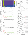
Figure 3. RF dynamics of an off-center Y-neuron.
Similar plots as for the Y-neuron in Fig. 1. Number of presentations of each spot 115.
Figure 4
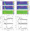
Figure 4. RF dynamics of a lagged on-center X-neuron.
Similar plots as for the Y-neuron in Fig. 1. In (A), notice the initial suppression of the response. Number of presentations of each spot 70.
Figure 5
Figure 5. Principal components analysis (PCA) for example on-center Y and X neurons in Figs. 1 and 2 .
A, B, 1st and 2nd principal components, respectively, for the Y-neuron response data, i.e., contributions from terms with n = 1 and n = 2 in Eq. (3). C, Sum of contributions from two first principal components (and background activity) for Y neuron. D, Deviation between experimental results for Y neuron and PCA results in (C). Error ε (cf. Eq. 1) is 0.036. E–H, Same as (A)–(D) for the X-neuron response data. The deviation between experimental results and PCA results (G) corresponds to an error ε = 0.015.
Figure 6
Figure 6. Fits to center-surround (CS) model for example on-center Y and X neurons in Figs. 1 and 2 .
A, Experimental Y-neuron response data. B, Best fit to CS-model in Eq. (6) with non-parametric representation of A(ti) and B(ti). C, Deviation between experimental results (A) and CS model results in (B). Error ε (cf. Eq. 1) is 0.071. D, Fitted values of weight parameters A(ti), and B(ti), cf. Eq. (6), E–H, Same as (A)–(D) for the X-neuron response data. The deviation between experimental results (E) and CS model results (F) corresponds to an error ε = 0.040.
Figure 7
Figure 7. Fits to time-resolved DOG functions for example on-center Y and X neurons in Figs. 1 and 2 .
A, Experimental Y-neuron response data. B, Best fit to time-resolved DOG model in Eq. (4). C, Deviation between experimental results (A) and model results in (B). Error ε (cf. Eq. 1) is 0.016. D, Fitted values of weight parameters A(ti) and B(ti) for Y neuron. E, Fitted values of width parameters a(ti) and b(ti) for Y neuron. F, Time-resolved error εt (cf. Eq. 2) for Y neuron. G–L, Same as (A)–(F) for the X-neuron response data. The deviation between experimental results (G) and model results (H) corresponds to an error ε = 0.012. Note that the almost vertical lines in panels (D) and (J) signal a rapid growth of the fitted value of the weight parameter B to values beyond the maximum values of the y-axes. The almost vertical lines in panels (E) and (K) correspondingly signal a rapid growth of the width parameter b.
Figure 8
Figure 8. Fits to spatial part of sustained component of TS model for example on-center Y and X neurons in Figs. 1 and 2 .
A, Last part (t>125 ms) of experimental Y-neuron response data used in fit. B, Best fit to DOG model in Eq. (10) representing the spatial part of the sustained component in the TS-model. C, Deviation between experimental results (A) and model results in (B). Error ε (cf. Eq. 1) is 0.053. D–F, Same as (A)–(C) for the X-neuron. The deviation between experimental results (D) and model results (E) corresponds to an error ε = 0.019. The fitted parameter values (As, Bs, as, bs) from both fits are listed in Table 1.
Figure 9
Figure 9. Principal components analysis (PCA) of early part of response data (t<100 ms) for example on-center Y and X neurons in Figs. 1 and 2 .
A,B, 1st and 2nd principal components, respectively, for the Y-neuron response data, i.e., contributions from terms with n = 1 and n = 2 in Eq. (3). C, Sum of contributions from two first principal components (and background activity) for Y neuron. D, Deviation between experimental results for Y neuron and PCA results in (C). Error ε (cf. Eq. 1) is 0.044. E, Fitted transient temporal function Ft1(t) (Eq. 11, blue dashed line) to 1st temporal PCA component (blue solid line), and fitted transient temporal function Ft2(t) (Eq. 12, green dashed line) to 2nd temporal PCA component (green solid line) for early part ( t<97.5 ms) of Y-neuron data. F, Blue dashed line: Fitted DOG spatial functions (Eq. 10) to 1st spatial PCA component of early part (t<97.5 ms) of Y-neuron data (blue solid line). Green dashed line: Corresponding DOG function fit to the 2nd spatial PCA component (green solid line). The best fit of a DOG function (red dashed line) to the 1st spatial PCA component of the last part of the Y-neuron data is also shown (red line). G–L, Same as (A)–(F) for X-neuron response data. The deviation between experimental results and PCA results (I) corresponds to an error ε = 0.021.
Figure 10
Figure 10. Fits to transient-sustained (TS) model for example on-center Y and X neurons in Figs. 1 and 2 .
A, Experimental Y-neuron response data. B, Best fit to TS model in Eq. (14). C, Deviation between experimental results (A) and model results in (B). Error ε (cf. Eq. 1) is 0.029. D, Transient component only, i.e., R(t,d) = [Rbkg+Ft1(t)Gt1(d)+Ft2(t)Gt2(d))]+. E, Sustained component only, i.e., R(t,d) = [Rbkg+Fs(t)Gs(d)]+. F, Fitted transient temporal functions Ft1(t) (Eq. 11,blue line) and Ft2(t) (Eq. 12, green line), and sustained temporal function Fs(t) (Eq. 13, red line) for Y-neuron. G, Fitted transient spatial functions Gt1(d) (blue line) and Gt2(d) (green line), and sustained spatial function Gs(d) (red line) for Y-neuron. All spatial functions are modeled as DOGs, cf. Eq. (10). H–N, Same as (A)–(G) for the X-neuron response data. The deviation between experimental results (H) and model results (I) corresponds to an error ε = 0.022. The fitted parameter values from both fits are listed in Table 1.
Figure 11
Figure 11. Predicted spatiotemporal impulse-response function DTS(t,r), cf. Eq.(16), for the transient-sustained (TS) model for example on-center Y and X neurons in Figs. 1 and 2 .
All model parameters correspond to the fit depicted in Fig. 10 and are listed in Table 1. A. Predicted impulse-response function for full TS-model for Y neuron. B. Contribution from transient part (ft1(t) gt1(r)+ft2(t) gt2(r)). C. Contribution from sustained part (fs(t) gs(r)). DF. Same as (A)–(C) for the X-neuron. Notice that (i) the color scale in C and F differ from the scale in the other corresponding color maps and (ii) that the negative response for the Y-neuron has been truncated at the value −50 spikes/s/deg2 in panels A and B.
Figure 12
Figure 12. Predicted ‘one-dimensional impulse response’, i.e., impulse response for long and thin bars, for the transient-sustained (TS) model for example on-center Y and X neurons in Figs. 1 and 2 .
This impulse-response function of the form given in Eq. (16), but with the spatial functions gm(r) replaced by the function gbar,m(x) listed in Eq. (21). The test bar in the example has a length L = 10 deg. All model parameters correspond to the fit depicted in Fig. 10 and are listed in Table 1. A. Predicted receptive-field function for full TS-model for Y neuron. B. Contribution from transient part (ft1(t) gbar,t1(x)+ft2(t) gbar,t2(x)). C. Contribution from sustained part (fs(t) gbar,s(x)). DF. Same as (A)–(C) for the X-neuron. Notice that (i) the color scale in C and F differ from the scale in the other corresponding color maps and (ii) that the negative response for the Y-neuron has been truncated at the numerical value −100 spikes/s/deg in panels A and B.
Figure 13
Figure 13. Fit of sustained-only model to the response data of the lagged cell in Fig. 4 .
A, Experimental data. B, Best fit to sustained-only model in Eq. (15). C, Deviation between experimental results (A) and model results in (B). Error ε (cf. Eq. 1) is 0.086.

Similar articles

Cited by

References

    1. Breitmeyer BG. Simple reaction time as a measure of the temporal response properties of transient and sustained channels. Vision Res. 1975;15:1411–1412. - PubMed
    1. Marr D, Poggio T. A computational theory of human stereo vision. Proc R Soc Lond B Biol Sci. 1979;204:301–328. - PubMed
    1. Ringach DL, Hawken MJ, Shapley R. Dynamics of orientation tuning in macaque primary visual cortex. Nature. 1997;387:281–284. - PubMed
    1. Bredfeldt CE, Ringach DL. Dynamics of spatial frequency tuning in macaque V1. J Neurosci. 2002;22:1976–1984. - PMC - PubMed
    1. Menz MD, Freeman RD. Stereoscopic depth processing in the visual cortex: a coarse-to-fine mechanism. Nat Neurosci. 2003;6:59–65. - PubMed

Publication types