The effect of noise correlations in populations of diversely tuned neurons

Abstract

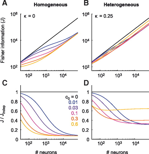
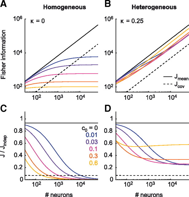
The amount of information encoded by networks of neurons critically depends on the correlation structure of their activity. Neurons with similar stimulus preferences tend to have higher noise correlations than others. In homogeneous populations of neurons, this limited range correlation structure is highly detrimental to the accuracy of a population code. Therefore, reduced spike count correlations under attention, after adaptation, or after learning have been interpreted as evidence for a more efficient population code. Here, we analyze the role of limited range correlations in more realistic, heterogeneous population models. We use Fisher information and maximum-likelihood decoding to show that reduced correlations do not necessarily improve encoding accuracy. In fact, in populations with more than a few hundred neurons, increasing the level of limited range correlations can substantially improve encoding accuracy. We found that this improvement results from a decrease in noise entropy that is associated with increasing correlations if the marginal distributions are unchanged. Surprisingly, for constant noise entropy and in the limit of large populations, the encoding accuracy is independent of both structure and magnitude of noise correlations.

Figure 1.

Illustration of the calculation of the linear Fisher information. A–D, Terms related to correlation structure. A, Matrix of correlation coefficients. The population has a limited range correlation structure. The correlation coefficient of two neurons depends only on the difference between their preferred directions. B, Covariance matrix. Variances are equal to mean spike counts. C, Correlation structure r. This corresponds to a single slice through the correlation coefficient matrix shown in A. D, Fourier transform of correlation structure shown in C. This is the power spectrum of the noise after normalizing to unit variances. E–I, Terms related to tuning curves in homogeneous population model. E, The tuning curves of the neurons. For clarity, one tuning curve (with preferred direction ϕ = 0) is highlighted. F, Average population response for θ = 0 given by f_j = f(−ϕ_j). All the following panels are evaluated at θ = 0. G, Normalized derivative g of the tuning curve. It looks flipped about the y-axis because g_j = f′ (−ϕ_j)/σ(−ϕ_j) and f′ is not symmetric. H, Power spectrum of normalized derivatives shown in G. I, Signal-to-noise ratio of individual Fourier components. J_mean is the sum over these terms. J–N, Terms related to tuning curves in heterogeneous population model. The panels are analogous to E–I. J, The tuning curves of the neurons. The average firing rate over all neurons and conditions is the same as for the homogeneous population. The tuning curve of one neuron is highlighted. K, Average population response for stimulus θ = 0. Because each neuron has a different peak amplitude, the population hill looks scattered around the mean tuning curve. Note that this scatter does not reflect noise. L, Normalized tuning curve derivatives g. M, Power spectrum of normalized tuning curve derivatives shown in L. Note that there is substantial power also in the higher frequencies (compare with H). N, Signal-to-noise ratio of all Fourier components.

Figure 2.

A, Fisher information as a function of population size in a homogeneous population of neurons (black line, independent population; colored lines, correlated populations; see legend in C). B, Same as in A but for heterogeneous population of neurons (κ = 0.25). C, Fisher information relative to independent population (J/J_indep) for a homogeneous population. D, Same as in C but for heterogeneous population of neurons.

Figure 3.

Relative contributions of J_mean and J_cov. The panels are analogous to those of Figure 2. The solid lines represent J_mean; the dashed lines represent J_cov. Colors represent different levels of correlation (see legend in C). A, J_mean and J_cov as a function of population size in a homogeneous population of neurons. B, Same as in A but for heterogeneous population of neurons (κ = 0.25). C, J_mean and J_cov for a homogeneous population relative to the total Fisher information of an independent population. D, Same as in C but for heterogeneous population of neurons.

Figure 4.

A, Relative J_mean as a function of correlation strength (c₀) in a homogeneous population of neurons (different colors indicate population sizes). B, Same as in A but for heterogeneous population of neurons (κ = 0.25). C, Relative J_cov in homogeneous population. D, Relative J_cov in heterogeneous population.

Figure 5.

Maximally detrimental level of correlations, c_min. This is the minimum of the curves in Figure 4B. Inset, The inverse of c_min is proportional to $\sqrt{n}$ (i.e., c_min decreases as O(1/$\sqrt{n}$)).

Figure 6.

Asymptotic (large n limit) Fisher information relative to independent population. A, Relative J_mean (black line, homogeneous population; colored lines, degree of heterogeneity, κ). Asymptotically, increased correlations always increase encoding accuracy (unless the neurons are independent). B, Relative J_cov is unaffected by heterogeneity in our model.

Figure 7.

MLE attains the Cramér–Rao bound. A, Efficiency of MLE relative to Fisher information for homogeneous population of neurons. The colors indicate different levels of correlation. B, As in A but for heterogeneous population.

Figure 8.

Fisher information for other types of tuning curve heterogeneity. A, J_mean for populations with random tuning widths. B, J_mean for populations with tuning parameters (baseline, amplitude, and width) sampled with replacement from a dataset of 408 orientation tuning curves from monkey V1. C, J_cov for populations with random tuning widths. D, J_cov for populations with all tuning parameters variable.

Figure 9.

Changing correlations affects noise entropy. The top row shows marginal distributions; the bottom row shows isoprobability contours (2σ from the mean) of two-dimensional joint distributions. A, An uncorrelated Gaussian distribution with σ = 1. B, Gaussian distribution with correlation coefficient r = 0.8 and marginals equal to the distribution in A (σ = 1). Its entropy (which is linearly related to the area enclosed by the ellipse) is 0.5 bits smaller than that of the distribution in A. C, Gaussian distribution with the same correlation coefficient and the same entropy as that in A. Its marginal SD is ≈30% larger (σ = 1.29) as that in A. Note that the ellipse has the same area as the circle in A.

Figure 10.

Effect of limited range correlations under constant noise entropy. A, Differential entropy (relative to an independent population and normalized by the number of neurons) as a function of correlation strength, c₀. B, Fano factor necessary to maintain constant noise entropy when increasing correlation strength. C, Linear Fisher information, J_mean, as a function of population size in heterogeneous populations with identical noise entropy (identical across different levels of correlation for the same n). Analogous to Figure 3B. D, J_mean relative to independent population (as in Fig. 3D).

Figure 11.

Relative J_mean for different correlation strengths under the constraint of constant noise entropy. A, Homogeneous population, κ = 0. B, Heterogeneous population, κ = 0.25. Asymptotically (n → ∞), the relative J_mean converges to κ.

Figure 12.

Dependence of OLE on correlations. Heterogeneous populations (κ = 0.25) are considered. This is similar to Figure 4. Dashed lines, J_mean; solid lines, OLE. The colors represent different population sizes (see legend in B). A, J_mean and the efficiency (inverse of the mean squared error) of the OLE relative to J_mean of an independent population. B, Zoomed-in version of A.

References

1. Abbott LF, Dayan P. The effect of correlated variability on the accuracy of a population code. Neural Comput. 1999;11:91–101. - PubMed
1. Bair W, Zohary E, Newsome WT. Correlated firing in macaque visual area MT: time scales and relationship to behavior. J Neurosci. 2001;21:1676–1697. - PMC - PubMed
1. Berens P, Ecker AS, Gerwinn S, Tolias AS, Bethge M. Reassessing optimal neural population codes with neurometric functions. Proc Natl Acad Sci U S A. 2011;108:4423–4428. - PMC - PubMed
1. Bethge M, Rotermund D, Pawelzik K. Optimal short-term population coding: when Fisher Information fails. Neural Comput. 2002;14:2317–2351. - PubMed
1. Cohen MR, Maunsell JH. Attention improves performance primarily by reducing interneuronal correlations. Nat Neurosci. 2009;12:1594–1600. - PMC - PubMed
Publication types
LinkOut - more resources