Understanding the structural ensembles of a highly extended disordered protein

Abstract

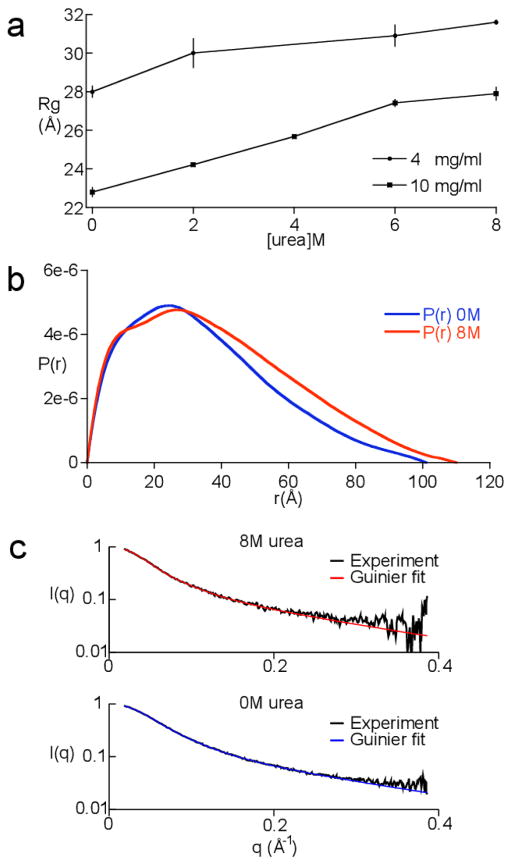
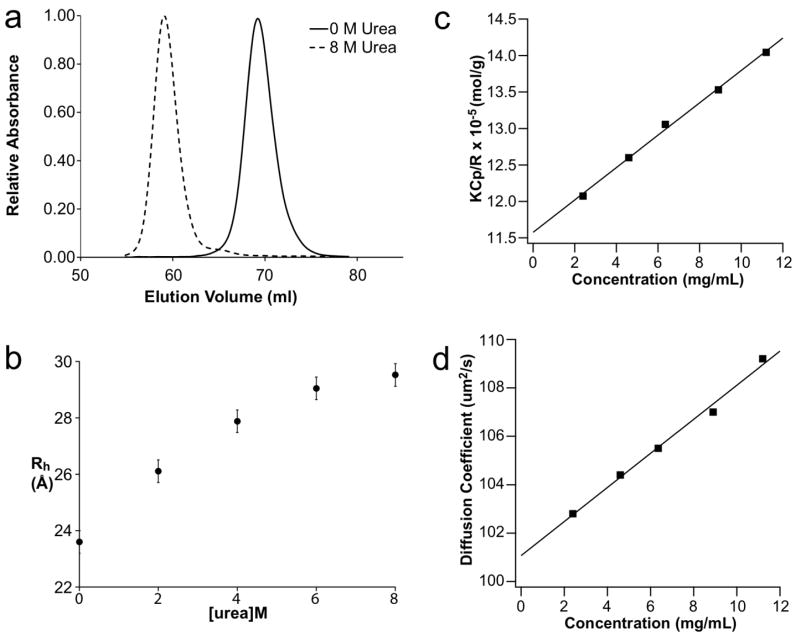
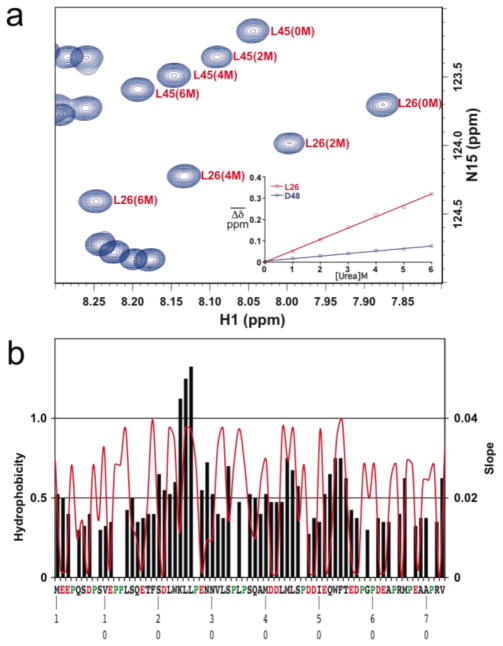
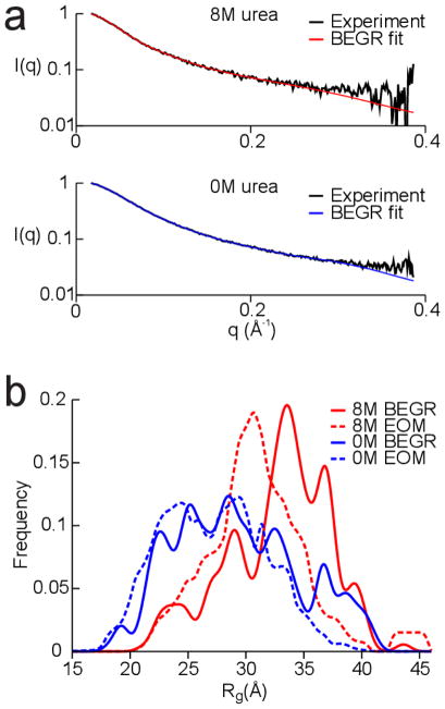
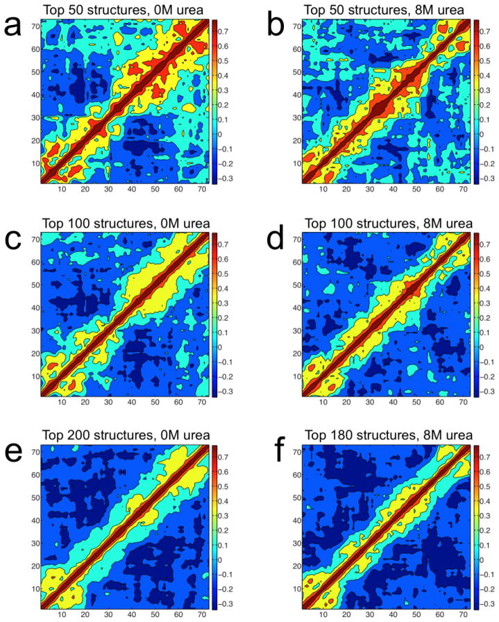
Developing a comprehensive description of the equilibrium structural ensembles for intrinsically disordered proteins (IDPs) is essential to understanding their function. The p53 transactivation domain (p53TAD) is an IDP that interacts with multiple protein partners and contains numerous phosphorylation sites. Multiple techniques were used to investigate the equilibrium structural ensemble of p53TAD in its native and chemically unfolded states. The results from these experiments show that the native state of p53TAD has dimensions similar to a classical random coil while the chemically unfolded state is more extended. To investigate the molecular properties responsible for this behavior, a novel algorithm that generates diverse and unbiased structural ensembles of IDPs was developed. This algorithm was used to generate a large pool of plausible p53TAD structures that were reweighted to identify a subset of structures with the best fit to small angle X-ray scattering data. High weight structures in the native state ensemble show features that are localized to protein binding sites and regions with high proline content. The features localized to the protein binding sites are mostly eliminated in the chemically unfolded ensemble; while, the regions with high proline content remain relatively unaffected. Data from NMR experiments support these results, showing that residues from the protein binding sites experience larger environmental changes upon unfolding by urea than regions with high proline content. This behavior is consistent with the urea-induced exposure of nonpolar and aromatic side-chains in the protein binding sites that are partially excluded from solvent in the native state ensemble.

Fig. 1

SAXS data for p53TAD. a. R_g values for p53TAD at 0, 2, 4, 6, and 8 M urea. R_g values are shown for 4 and 10 mg/ml samples. b. Internuclear distance distributions for 4 mg/ml p53TAD samples in 0 (blue curve) and 8 M (red curve) urea. c. Fits to the scattering curves in reciprocal space. Plot shows the scattering intensity, I(q), as a function of the scattering vector, q. The data is shown in black and the fits are shown in blue and red for 0 and 8 M urea, respectively.

Fig. 2

Hydrodynamic radii from size exclusion chromatography and static and dynamic light scattering. a. Chromatographic traces at 0 and 8 M urea. b. R_h values calculated at the different urea concentrations. c. The Debye Ratio (KCp/R) versus p53TAD concentration. d. Mutual diffusion coefficient D_m vs. p53TAD concentration. For c and d, the squares are individual measurements and the solid lines are linear fits through these data. According to eqns (2) and (4), the intercepts and slopes of these curves yield the following parameters for p53TAD: MW = 8.6 kDa, B₂₂ = 11.2 x 10⁻⁴ mL mol/g², D₀ = 101.1 ± 0.3 μm²/s, and R_h = 23.9 ± 0.1 Å.

Fig. 3

Residue specific chemical shift changes as a function of urea. a. Overlay of a selected region from the ¹H-¹⁵N HSQC spectra at 0, 2, 4, and 6 M urea. Inset shows plots for two residues (L26 and D48). b. black bars show slope values and red line shows a hydrophobicity plot.

Fig. 4

Fitting the SAXS data using the BEGR ensembles. a. Plot of the scattering intensity decay, I(q), as a function of the scattering vector, q. Black lines show the SAXS data for 0 M and 8 M urea and blue and red lines show the fits using the BEGR ensembles. b. Plot of the R_g distribution for structures from the BEGR (solid lines) and EOM (dashed lines) ensembles.

Fig. 5

Correlation plots for number of neighbors using the top weighted structures from the 0 and 8 M BEGR ensembles. The observed correlations vary from −0.3 (dark blue) to 0.7 (dark red) and a scale bar is shown to the right of each plot. Amino acid position is shown on both axes. Correlation plots for a) 50, c) 100, and e) 200 top weighted structures from a total of 227 structures in the 0 M BEGR ensemble, representing representing 50.0%, 78.5%, and 99.5% of the total weight, respectively. Correlation plots for the b) 50, d) 100, and f) 180 top weighted structures from a total of 189 structures in the 8 M BEGR ensemble, representing 55.4%, 83.2%, and 99.8% of the total weight, respectively.

References

1. Wright PE, Dyson HJ. J Mol Biol. 1999;293:321–331. - PubMed
1. Daughdrill GW, Pielak GJ, Uversky VN, Cortese MS, Dunker AK. In: Protein Folding Handbook. Buchner J, Kiefhaber T, editors. Vol. 3. WILEY-VCH; Darmstadt: 2005. pp. 275–357.
1. Vendruscolo M. Curr Opin Struct Biol. 2007;17:15–20. - PubMed
1. Uversky VN. Eur J Biochem. 2002;269:2–12. - PubMed
1. Uversky VN. Protein Sci. 2002;11:739–756. - PMC - PubMed
Publication types