Coexistence of lateral and co-tuned inhibitory configurations in cortical networks

Abstract

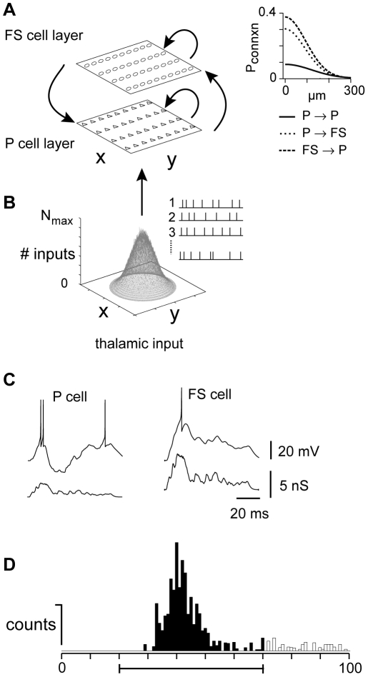
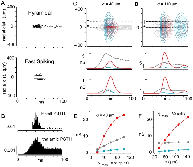
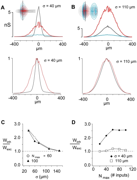
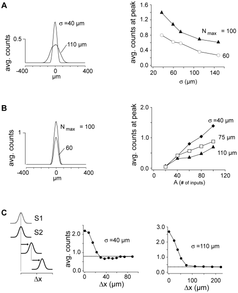
The responses of neurons in sensory cortex depend on the summation of excitatory and inhibitory synaptic inputs. How the excitatory and inhibitory inputs scale with stimulus depends on the network architecture, which ranges from the lateral inhibitory configuration where excitatory inputs are more narrowly tuned than inhibitory inputs, to the co-tuned configuration where both are tuned equally. The underlying circuitry that gives rise to lateral inhibition and co-tuning is yet unclear. Using large-scale network simulations with experimentally determined connectivity patterns and simulations with rate models, we show that the spatial extent of the input determined the configuration: there was a smooth transition from lateral inhibition with narrow input to co-tuning with broad input. The transition from lateral inhibition to co-tuning was accompanied by shifts in overall gain (reduced), output firing pattern (from tonic to phasic) and rate-level functions (from non-monotonic to monotonically increasing). The results suggest that a single cortical network architecture could account for the extended range of experimentally observed response types between the extremes of lateral inhibitory versus co-tuned configurations.

Figure 1. Model schematics.

A, Left, Network is a sheet of neurons with a pyramidal (P) and a fast spiking (FS) cell layer. Arrows depict connections between and across layers. Right, Gaussian connectivity profiles were fit to experimental data (not shown) for connection probability (abscissa) versus intersomatic distance (ordinate). See Results for parameter values. B, The average number of inputs that any P or FS cell received from the thalalmus was Gaussian distributed, with peak value of N_max. Inset, example thalamic cell trains. C, Thalamic conductance input (bottom) and associated voltage response (top) of representative P (left) and FS (right) cells. D, Post-stimulus time histogram compiled from spike trains of P cells in the center of the network. Firing was quantified as the number of counts within a 50 ms time interval from the stimulus onset divided by the number of trials (bar, filled portion of the histogram).

Figure 2. Spatiotemporal profiles of firing and synaptic conductances.

A, Spike rasters obtained with simulations on a 2 dimensional network of P (top) and FS (bottom) cells. Rasters are arranged according to neurons' symmetric radial distance from the center of the network. Each line is from a representative neuron at a given radial distance and is compiled from 50 sweeps. B, Post-stimulus time histograms of P cell (top) and thalamic cell (bottom) populations. C, top, Normalized contour plots showing spatiotemporal profiles of thalamic (gray), recurrent excitatory (cyan), and FS inhibitory synaptic conductances (red) evoked in P cells. Temporal profiles of conductances evoked in a P cell at (*, middle) and away (†, bottom) from the center. Thalamic input was narrow (σ = 40 µm). D, same as in C but for a wider thalamic input (σ = 110 µm). E, left, plot of peak conductances (color code as above) vs the number of thalamic inputs N_max for σ = 40 µm. F, peak conductance vs σ for N_max  = 60.

Figure 3. Spatial profiles of synaptic components.

A, Top, spatial profiles of thalamic (gray), recurrent excitatory (cyan), and FS inhibitory (red) conductances evoked in P cells at different radial distances (abscissa) from the center for σ = 40 µm. Dotted line in inset shows where on the contour plots the spatial profiles were obtained. Bottom, normalized profiles for composite excitatory (black, thalamic + recurrent) and inhibitory (red) conductances generated in P cells B, Similar profiles for σ = 110 µm C, ratio of inhibitory to excitatory spatial profile half-widths, w_inh/w_exc, vs σ for N_max = 60 and 100. D, w_inh/w_exc vs. N_max for σ = 40 µm and 110 µm.

Figure 4. Firing responses of P cells.

A, left, Average number of action potentials evoked in the first 50 ms of stimulus of cells at different radial distances from the center (abscissa) for broad (σ  = 110 µm) and narrow (σ  = 40 µm) thalamic inputs (N_max  = 60). Right, plot of counts at the peak of the profiles vs σ for N_max = 60 and 100. B, left, spatial profile of average counts for N_max = 60 and 100 with σ fixed at 40 µm. Right, plot of peak counts vs N_max for σ  = 40, 75 and 110 µm. C, left, networks stimulated with 2 inputs (S1 & S2), with S2 at different positions (Δx) in the network. N_max = 60. Middle, average counts evoked vs Δx for narrow input (σ = 40 µm). Right, average counts vs Δx for broad input (σ = 110 µm).

Figure 5. Activity in the feedforward network. A

, Schematic of network architecture. Inhibitory cells innervate excitatory cells; both receive spatially distributed inputs (I_thal) from a presynaptic population of cells. B, Procedure for calculating spatial profiles of excitatory (I_exc) and inhibitory (I_inh) inputs to excitatory cells. C, top, ratio of I_inh to I_exc widths, w_inh/w_exc, as a function of N_max and σ. N_max is normalized (divided) by the minimum current needed to evoke excitatory cell firing and σ is normalized by the standard deviation of the inhibitory spread (σ_inh of P_inh in B). Intersection with unitary plane (purple) gives values of N_max and σ where I_exc and I_inh are perfectly co-tuned. Bottom, plot of w_inh/w_exc vs σ at N_max = 3 (corresponding to dotted line at Top). D, Peak excitatory (gray) and inhibitory (red) current plotted against N_max and σ. Purple line corresponds to values of N_max and σ that produced perfect co-tuning in C. Bottom, plot of peak excitatory (blue) and inhibitory (red) vs N_max for σ = 1.6 (corresponding to dotted line at top).

Figure 6. Variation of firing with input.

Rate models were used to calculate the firing in the σ σ – N_max space (see Methods). The network had a single spatial dimension with connection profiles derived from in vitro data. A, B, spatiotemporal pattern of excitatory cell firing rates for narrow input (σ = 40 µm, A and broad input (σ = 120 µm, B). N_max = 20 for both panels. C, left, ratio of widths of inhibitory to excitatory current input to excitatory cells vs. N_max and σ. Purple line denotes co-tuning. Blue and yellow circles correspond to values of N_max and σ used in A and B, respectively. Right, peak excitatory (gray) and inhibitory (red) current (c.f. Fig. 5D). Purple line denotes perfect co-tuning. D, mean firing rate (calculated over the first 50 ms) for the center excitatory cell vs. N_max and σ.

Figure 7. Response trajectories in the σ– N_max space.

A, top, input to auditory thalamus (MGv) is relayed to cortex as a Gaussian activity profile parameterized by N_max and σ. Middle, transfer functions for specific stimulus-response trajectories. Curves were Naka-Rushton functions (eqn 9) with parameter values: M = 1000, n = 5, θ = 0.4 (N_max); M = 75, n = 4, θ = 0.5 (σ); the curve for broad σ (dashed) was additionally shifted up by 75 µm. A single graded stimulus generates concurrent increases in N_max and σ of the Gaussian input profiles (schematized at bottom). B, top, excitatory cell firing rate (F_exc) vs. N_max and σ. Solid and dashed curves correspond to the transfer functions in A, middle. Gray line denotes perfect co-tuning (c.f. Fig. 6B,C). Bottom, F_exc vs. stimulus intensity.

References

1. Volkov IO, Galazjuk AV. Formation of spike response to sound tones in cat auditory cortex neurons: interaction of excitatory and inhibitory effects. Neuroscience. 1991;43:307–321. - PubMed
1. Wang X, Lu T, Snider RK, Liang L. Sustained firing in auditory cortex evoked by preferred stimuli. Nature. 2005;435:341–346. - PubMed
1. Schreiner CE, Mendelson JR, Sutter ML. Functional topography of cat primary auditory cortex: representation of tone intensity. Exp Brain Res. 1992;92:105–122. - PubMed
1. Calford MB, Semple MN. Monaural inhibition in cat auditory cortex. J Neurophysiol. 1995;73:1876–1891. - PubMed
1. Sadagopan S, Wang X. Nonlinear spectrotemporal interactions underlying selectivity for complex sounds in auditory cortex. J Neurosci. 2009;29:11192–11202. - PMC - PubMed
Publication types