Systematic analysis of protein pools, isoforms, and modifications affecting turnover and subcellular localization

Abstract

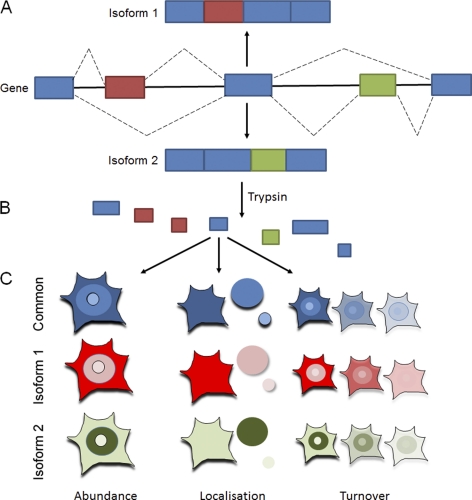
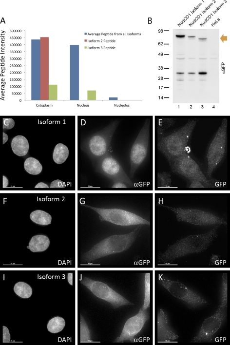
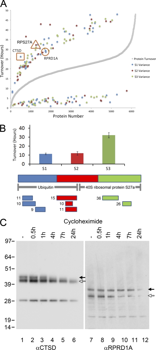
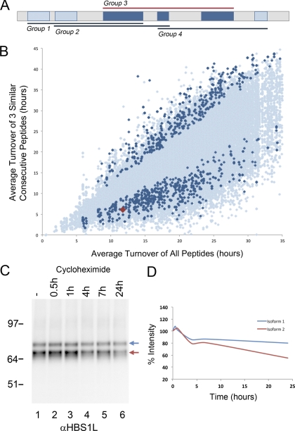
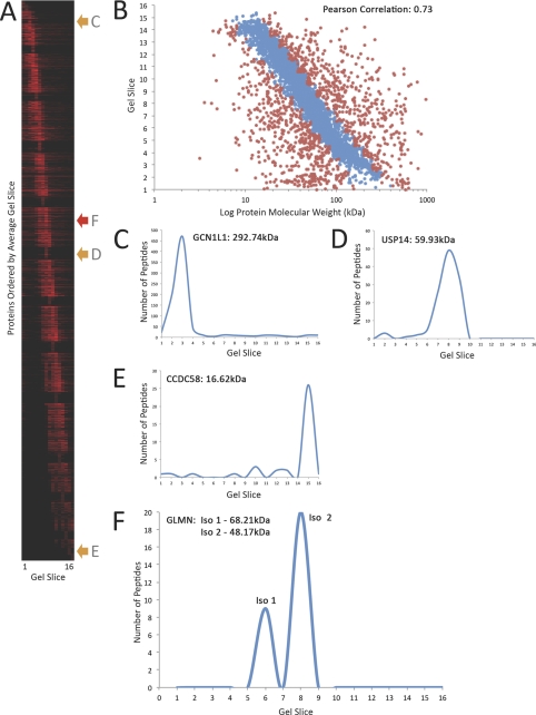
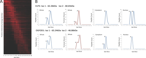
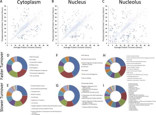
In higher eukaryotes many genes encode protein isoforms whose properties and biological roles are often poorly characterized. Here we describe systematic approaches for detection of either distinct isoforms, or separate pools of the same isoform, with differential biological properties. Using information from ion intensities we have estimated protein abundance levels and using rates of change in stable isotope labeling with amino acids in cell culture isotope ratios we measured turnover rates and subcellular distribution for the HeLa cell proteome. Protein isoforms were detected using three data analysis strategies that evaluate differences between stable isotope labeling with amino acids in cell culture isotope ratios for specific groups of peptides within the total set of peptides assigned to a protein. The candidate approach compares stable isotope labeling with amino acids in cell culture isotope ratios for predicted isoform-specific peptides, with ratio values for peptides shared by all the isoforms. The rule of thirds approach compares the mean isotope ratio values for all peptides in each of three equal segments along the linear length of the protein, assessing differences between segment values. The three in a row approach compares mean isotope ratio values for each sequential group of three adjacent peptides, assessing differences with the mean value for all peptides assigned to the protein. Protein isoforms were also detected and their properties evaluated by fractionating cell extracts on one-dimensional SDS-PAGE prior to trypsin digestion and MS analysis and independently evaluating isotope ratio values for the same peptides isolated from different gel slices. The effect of protein phosphorylation on turnover rates was analyzed by comparing mean turnover values calculated for all peptides assigned to a protein, either including, or excluding, values for cognate phosphopeptides. Collectively, these experimental and analytical approaches provide a framework for expanding the functional annotation of the genome.

Fig. 1.

Alternative splicing leading to protein isoforms. A, A single gene can encode multiple proteins because of alternative splicing. After transcription of a gene, exons of the resultant RNA can be reconnected in multiple ways during RNA splicing, resulting in the translation of protein isoforms, with red and green areas signifying differences between the isoforms. B, Protein isoforms represent several different forms of a protein and have a largely shared sequence, however small differences occur. Mass spectrometery can be used to identify both common peptides shared by all isoforms and specific peptides (shown in red and green) that are unique to each isoform. C, Using these identified peptides it is possible to extract abundance, localization, and turnover information for a protein by using either shared peptides or isoform specific peptides.

Fig. 2.

NUDCD1 protein isoform identification and localization from peptide intensities. Identification of NudCD1, NudC domain-containing protein 1. A, Chart showing intensity (y axis) in different cellular compartments (x axis) for three peptides. The blue series provides average intensity of common peptides shared between isoforms of NudCD1. Remaining series show intensity of MLYLQGWSMPAVAEVK (isoform 2 peptide - red) and YNQDTALGKPR (isoform 3 peptide - green). The isoform 3 specific peptide has intensity in both cytoplasmic and nuclear compartments (∼3:2 cytoplasmic/nuclear), and the isoform 2 peptide shows exclusively cytoplasmic signal. B, HeLa cells expressing GFP used to detect isoforms of NudCD1. Upper bands on the Western blot (orange arrow) show three protein isoforms recognized, migrating at the predicted molecular weights of NudCD1 isoforms. Fluorescence microscopy analysis of the HeLa cells expressing the respective GFP-fusion proteins was performed using both antibody to GFP (panels D, G, and J), and direct GFP fluorescence (panels E, H, and K). NudCD1 Isoform 1 shows nuclear accumulation in panels D and E, NudCD1 isoform 2 shows predominantly cytoplasmic accumulation in panels G and H and both cytoplasmic and nuclear accumulation is shown of NudCD1 isoform 3 in panels J and K.

Fig. 3.

Protein isoform identification from protein sequence segmentation. A, Graph showing all proteins (x axis) (ordered by average protein turnover) plotted against turnover in hours (y axis). Gray series shows average turnover for each protein. Blue, red, and green series highlight segments of proteins that have a variance of 70% or more compared with average protein turnover. B, Chart shows the three equal segments of RPS27A, Ubiquitin-40S ribosomal protein S27a, plotted on x axis against average turnover on y axis. Peptides for each segment (examples shown underneath) have significantly different turnover in carboxyl terminal segment 3 compared with segments 1 and 2. RPS27A protein is expressed as a precursor that is processed to yield ubiquitin. C, Further proteins tested were, CTSD - Cathepsin d- (shown in orange square in A) and RPRD1A - Regulation of nuclear pre-mRNA domain-containing protein 1A (shown in orange circle in A). Cycloheximide inhibition experiments were performed on HeLa cells to block protein synthesis and thus measure the rate of protein degradation. The Western blot for CTSD shows a band at predicted molecular weight of 44.55 kDa (white arrow). Another, higher, band is visible (black arrow), which shows a faster turnover across the five timepoints (lanes 2–6). The second protein tested, RPRD1A, shows two bands on the Western blot, which correlate with the expected molecular weight of the known isoforms of RPRD1A (isoform 1 at 35.72kDa, isoform 2 at 32.92kDa and 31.63kDa). The upper band (black arrow, isoform 1) shows slower degradation over the timecourse (lanes 8–12) compared with the lower band (white arrow) (isoforms 2 and 3).

Fig. 4.

Protein isoform identification from consecutive peptide analysis. A, Groups of three consecutive peptides were identified and average turnover value of each group calculated. A linear representation of protein is shown, with highlighted regions indicating identified peptides. Any group showing a 20% variance in turnover from the average protein turnover is labeled as interesting (Group 3). B, Graph showing average protein turnover from all peptides (x axis) versus average turnover of three consecutive peptides from the protein (y-axis). Data points highlighted in blue indicate three consecutive peptides that all have a turnover that varies by 20% greater or less than the average protein turnover. Highlighted in red, is protein HBS1L, HBS1-like protein. C, Cycloheximide experiment was carried out to measure the degradation rate of HBS1L. Antibody for HBS1L detected two bands, consistent with expression of two isoforms (blue and red arrows). These bands correlate to the known isoforms of HBS1L (isoform 1 at 75.5 kDa (blue arrow), isoforms 2 and 3 at 70.13 kDa and 70.63 kDa (red arrow)). D, Quantitation of the two bands at multiple time points from 0.5–24 h (lanes 2–6) is shown on the graph. The percentage intensity is plotted on the y axis, across the timecourse on the x axis. Graph shows that the two putative isoforms of HBS1L differ in their degradation rates.

Fig. 5.

Protein migration study on gel fractionation. A, Heat map of the 16 gel slices (horizontally) is shown with every protein identified (vertically) ordered by the average gel slice the protein was found in. B, Graph showing predicted log protein molecular weight (x axis) against gel slice (y axis), indicating that proteins predictably migrated across the gel based on their molecular weights (Pearson Correlation: 0.73). Graphs C, D, and E highlight three examples of proteins, GCN1L1 (Translational activator GCN1), USP14 (Ubiquitin carboxyl-terminal hydrolase 14) and CCDC58 (Coiled-coil domain-containing protein 58) respectively, where the peptide count (y axis) is plotted against gel slice (x axis). These graphs show that the proteins migrate at different gel slices consistent with their molecular weight. F, Graph showing peptide count (y axis) plotted versus gel slice and molecular weight (x axis) for protein GLMN (Glomulin). The gel fractionation data indicate that this protein migrates at two gel slices, 6 and 8. GLMN, has in fact two known isoforms, isoform 1 at 68.21 kDa and isoform 2 at 48.17 kDa.

Fig. 6.

Protein isoform identification from gel fractionation. A, Heat map showing the 16 gel slices and their corresponding molecular weights (horizontally) for every protein identified (vertically) ordered by the average gel slice the protein was found in. This heat map was filtered to show only proteins that migrate at multiple gel slices. B, Two example proteins are shown, ELP3 (Elongator complex protein 3) and OGFOD1 (2-oxoglutarate and iron-dependent oxygenase domain-containing protein 1). The graphs on the left show peptide count (y axis) versus gel slice (x axis) as an aggregate for the whole cell, indicating that both ELP3 and OGFOD1 migrate at two separate gel slices. The cytoplasmic graph (top-middle-right) and nuclear graph (top-right) for ELP3 indicate that only one isoform is present in the Cytoplasm (A′), whereas both isoforms are detected in the Nucleus (A and A′). The turnover graph (top-middle-left), showing the turnover values detected (y axis), in each gel slice (x axis), indicates that both isoforms of ELP3 have a different turnover, i.e. 6 h (A) and 28 h (A′) respectively. In relation to OGFOD, the cytoplasmic graph (bottom-middle-right) and nuclear graph (bottom-right) show the isoform A is found in both the cytoplasm and nucleus, however isoform A′ is only found in the cytoplasm. The turnover graph (bottom-middle-left), showing the turnover values detected (y axis) in each gel slice (x axis), indicates that the two forms of the OGFOD1 protein at the different gel slices have different turnovers, i.e. 18.18 h (A) and 37.49 h (A′).

Fig. 7.

Correlation analysis of phosphopeptides with turnover. Graphs A, B, and C show the average protein turnover using nonphosphorylated peptides (x axis) against average protein turnover using both phosphorylated and nonphosphorylated peptides in each of the cytoplasmic, nuclear, and nucleolar compartments. Highlighted in blue are phosphorylated proteins that show a 1.5-fold change compared with the nonphosphorylated form of the protein. Comparison of graphs A (cytoplasm), B (nucleus), and C (nucleolus) show that the nucleolus has the greatest number of phosphorylated proteins compared with the cytoplasm and nucleus. The pie charts D, E, and F show the gene ontology analysis of the phosphorylate proteins that have a slower turnover in comparison with phosphorylated from and, similarly, pie charts G, H, and I show the gene ontology analysis of the phosphorylated proteins that have a faster turnover in comparison with the nonphosphorylated form.

References

1. Corthals G. L., Wasinger V. C., Hochstrasser D. F., Sanchez J. C. (2000) The dynamic range of protein expression: a challenge for proteomic research. Electrophoresis 21, 1104–1115 - PubMed
1. Hinkson I. V., Elias J. E. (2011) The dynamic state of protein turnover: It's about time. Trends Cell. Biol. 21, 293–303 - PubMed
1. Nesvizhskii A. I., Aebersold R. (2005) Interpretation of Shotgun Proteomic Data. Mol. Cell. Proteomics 4, 1419–1440 - PubMed
1. Rappsilber J., Mann M. (2002) What does it mean to identify a protein in proteomics? Trends Biochem. Sci. 27, 74–78 - PubMed
1. Godovac-Zimmermann J., Kleiner O., Brown L. R., Drukier A. K. (2005) Perspectives in spicing up proteomics with splicing. Proteomics 5, 699–709 - PubMed
Publication types
LinkOut - more resources