Individual subject classification for Alzheimer's disease based on incremental learning using a spatial frequency representation of cortical thickness data

Abstract

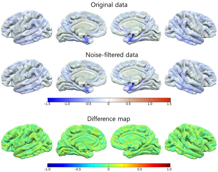
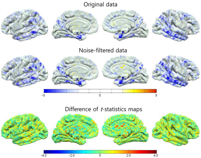
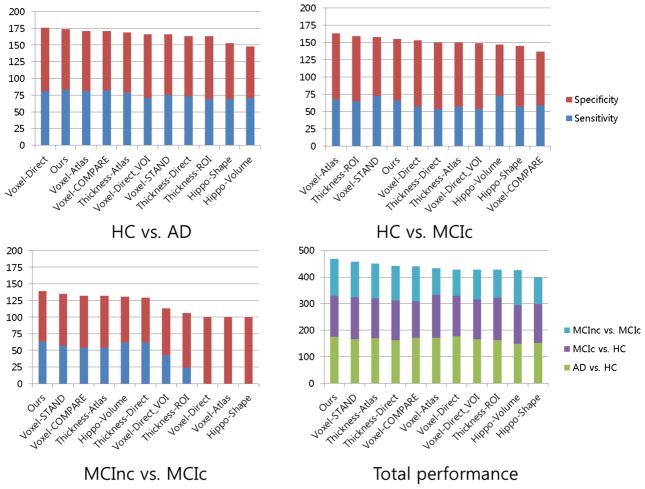
Patterns of brain atrophy measured by magnetic resonance structural imaging have been utilized as significant biomarkers for diagnosis of Alzheimer's disease (AD). However, brain atrophy is variable across patients and is non-specific for AD in general. Thus, automatic methods for AD classification require a large number of structural data due to complex and variable patterns of brain atrophy. In this paper, we propose an incremental method for AD classification using cortical thickness data. We represent the cortical thickness data of a subject in terms of their spatial frequency components, employing the manifold harmonic transform. The basis functions for this transform are obtained from the eigenfunctions of the Laplace-Beltrami operator, which are dependent only on the geometry of a cortical surface but not on the cortical thickness defined on it. This facilitates individual subject classification based on incremental learning. In general, methods based on region-wise features poorly reflect the detailed spatial variation of cortical thickness, and those based on vertex-wise features are sensitive to noise. Adopting a vertex-wise cortical thickness representation, our method can still achieve robustness to noise by filtering out high frequency components of the cortical thickness data while reflecting their spatial variation. This compromise leads to high accuracy in AD classification. We utilized MR volumes provided by Alzheimer's Disease Neuroimaging Initiative (ADNI) to validate the performance of the method. Our method discriminated AD patients from Healthy Control (HC) subjects with 82% sensitivity and 93% specificity. It also discriminated Mild Cognitive Impairment (MCI) patients, who converted to AD within 18 months, from non-converted MCI subjects with 63% sensitivity and 76% specificity. Moreover, it showed that the entorhinal cortex was the most discriminative region for classification, which is consistent with previous pathological findings. In comparison with other classification methods, our method demonstrated high classification performance in both categories, which supports the discriminative power of our method in both AD diagnosis and AD prediction.

Figure 1

Overview of the proposed classification method.

Figure 2

Visualization of eigenvectors for the LB operator on the left cortical surface mesh: h^k denotes the k^th eigenfunction. The value of the k^th eigenvector for large k changes periodically with a short cycle on the mesh.

Figure 3

2D illustration of LDA classification for two groups: LDA finds the coordinate axes which maximally separate the groups of a data set. In this figure, the axis w₁ for the data set better separates two groups than the axis w₂. Specifically, the mean difference between the groups is larger on w₁ than on w₂, while the variance within each group is smaller on w₁ than on w₂. LDA maximizes the between-class variance across the groups and minimizes the within-class variance for each group.

Figure 4

Accuracies of individual subject classifiers with respect to cut-off dimension F

Figure 5

Visualization of the mean difference of cortical thickness between AD and HC: The first and the second rows show the mean difference in the original data set and the noise-filtered data set, respectively. The third row visualizes the difference between the first and the second rows.

Figure 6

Comparison of t-statistics maps between the original and noise-filtered cortical thickness data: Statistically significant regions for the noise-filtered data subset (Dataset 1) were similar to those for the original one. The third row shows the difference of absolute t-statistics values at every vertex between the original and noise-filtered data sets. A warm color represents that the noise-filtered data subset is statistically more significant than the original one, while a cold color represents the opposite case. For more than 65% of the whole surface region, the noise-filtered data set has greater t-statistics values, which verifies that our noise removal scheme improves the results of statistical analysis.

Figure 7

Benchmark results for eleven classification methods, in which their performances were shown in the descending order. Our method received good evaluations in all classifications: it showed the highest performance in MCInc vs. MCIc classification and the second highest in HC vs. AD classification. In HC vs. MCIc classification, it was ranked in the fourth position. The benchmark results demonstrated that our classification exhibited high performance compared to other classification methods.

Figure 8

The discriminative regions in HC vs. AD classification, MCInc vs. MCIc classification, and HC vs. MCIc classification: Each figure visualizes the LDA axes on the atlas meshes.

Figure 9

Average accuracies of individual subject classifiers with respect to the number of used training subjects: The average accuracy of each classifier tended to increase in the number of used training subjects.

Figure 10

The computation times for training the HC vs. AD classifier in batch learning and incremental learning: We increased the size of our data up to (including) 13,000 by reusing the test data of Dataset 1. We separately measured the computation times for the incremental learning and the batch learning, excluding that for the feature vector construction. The computation time for incremental learning was constantly 1.4 seconds regardless of the cumulative size of training data since it is dependent on the size of new training data. On the other hand, the computation time of batch learning rapidly growing in the cumulative size of training data.

References

1. Anticevic A, Dierker DL, Gillespie SK, Repovs G, Csernansky JG, Essen DCV, Barch DM. Comparing surface-based and volume-based analyses of functional neuroimaging data in patients with schizophrenia. NeuroImage. 2008;41 (3):835–848. - PMC - PubMed
1. Bain LJ, Jedrziewski K, Morrison-Bogorad M, Albert M, Cotman C, Hendrie H, Trojanowski JQ. Healthy brain aging: A meeting report from the sylvan m. cohen annual retreat of the university of pennsylvania institute on aging. Alzheimer’s and Dementia. 2008;4 (6):443–446. - PMC - PubMed
1. Balakrishnama S, Ganapathiraju A. Linear discriminant analysis - a brief tutorial [online] 1998 Available: http://www.music.mcgill.ca/ich/classes/mumt61105/classifiers/ldatheory.pdf.
1. Belhumeur PN, Hespanha JP, Kriegman DJ. Eigenfaces vs. fisherfaces: Recognition using class specific linear projection. IEEE Transactions on Pattern Analysis and Machine Intelligence. 1997;19:711–720.
1. Bylesjø M, Rantalainen M, Cloarec O, Nicholson JK, Holmes E, Tryg J. Opls discriminant analysis: combining the strengths of pls-da and simca classification. Journal of Chemometrics. 2006;20 (8–10):341–351.
Publication types