Capturing inter-subject variability with group independent component analysis of fMRI data: a simulation study

Abstract

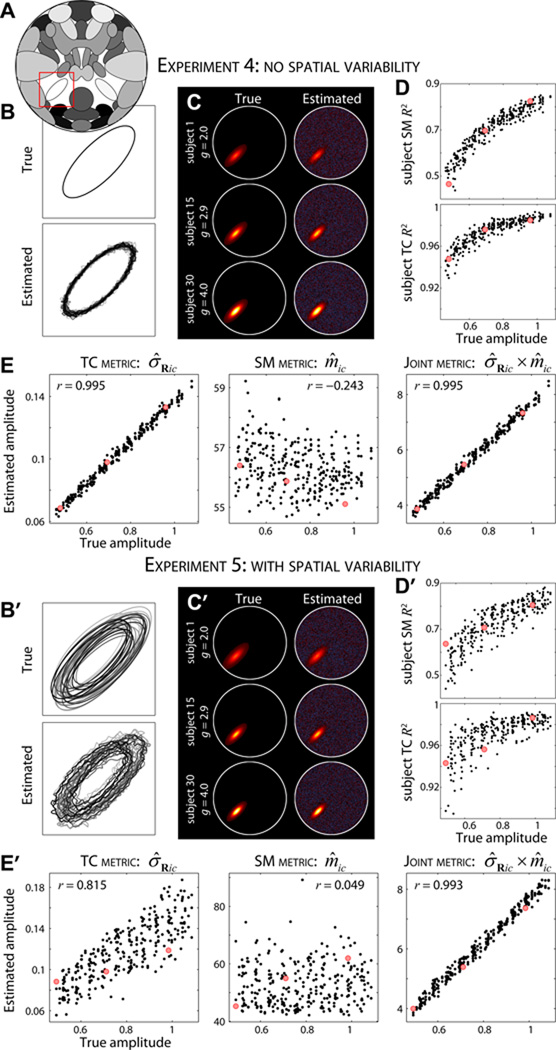
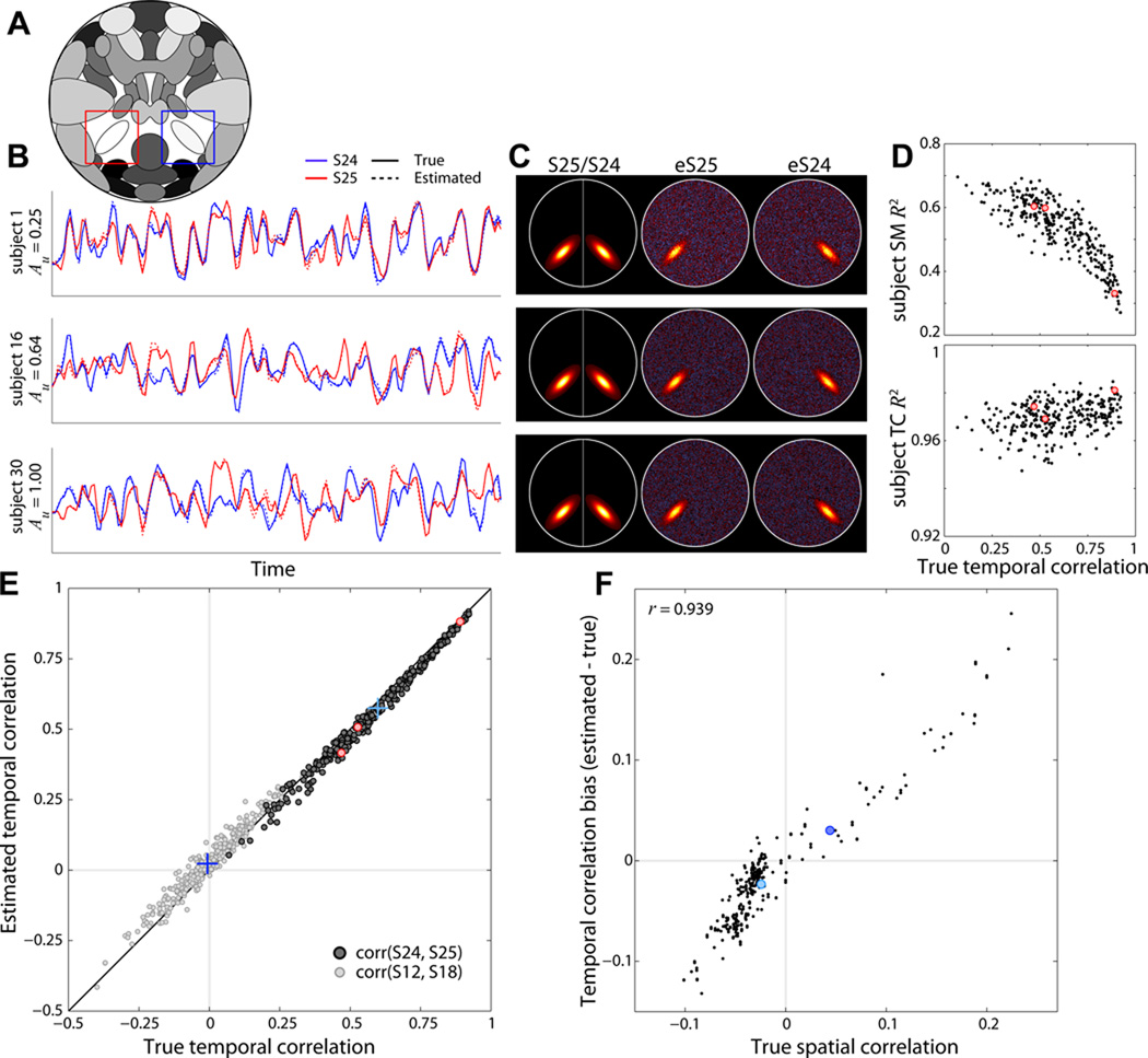
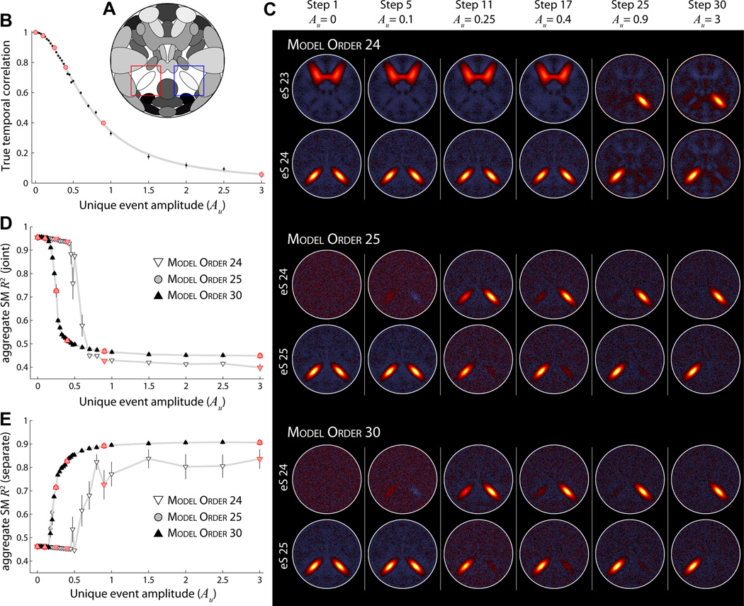
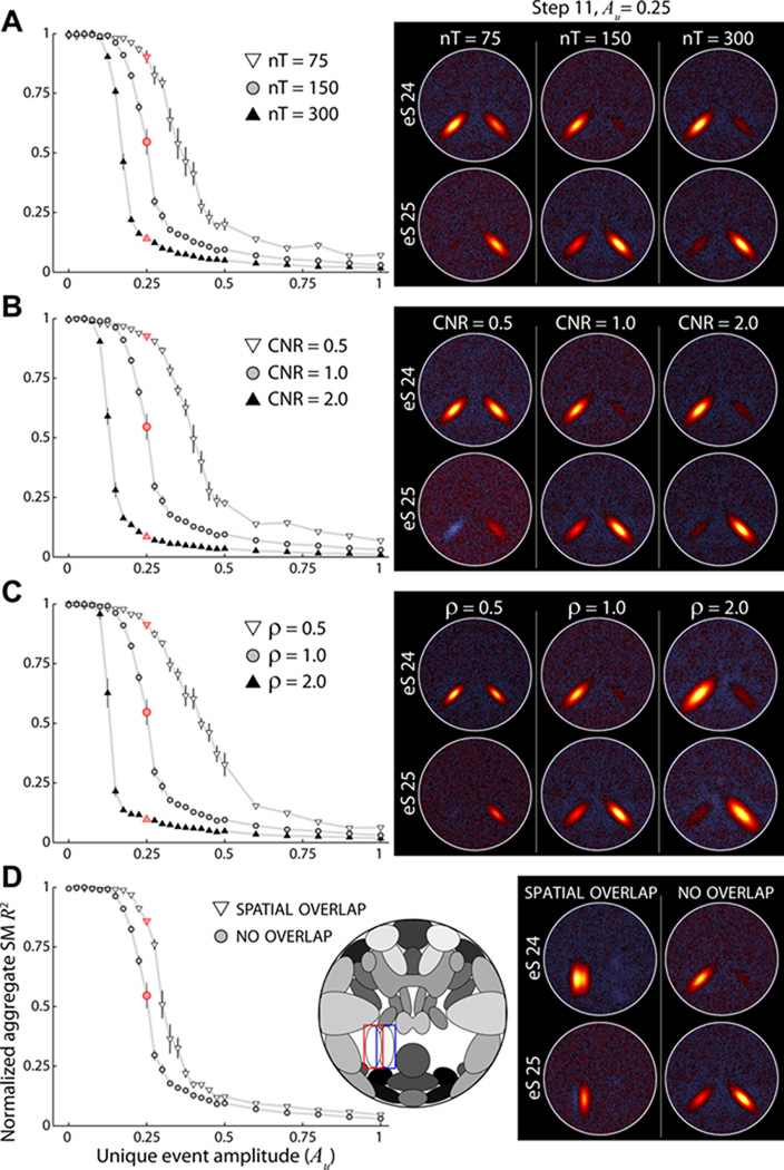
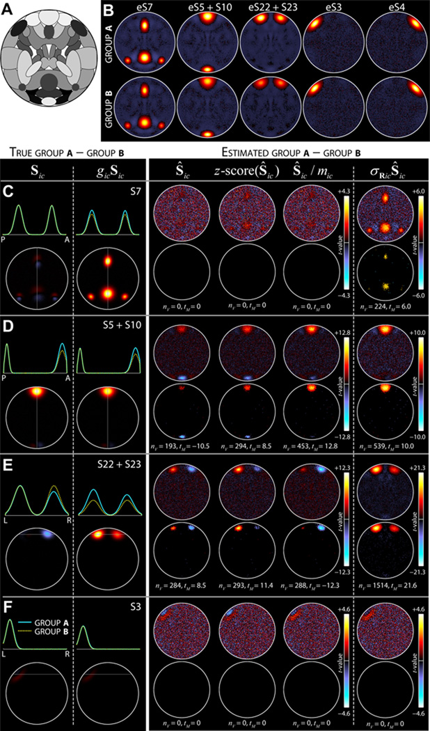
A key challenge in functional neuroimaging is the meaningful combination of results across subjects. Even in a sample of healthy participants, brain morphology and functional organization exhibit considerable variability, such that no two individuals have the same neural activation at the same location in response to the same stimulus. This inter-subject variability limits inferences at the group-level as average activation patterns may fail to represent the patterns seen in individuals. A promising approach to multi-subject analysis is group independent component analysis (GICA), which identifies group components and reconstructs activations at the individual level. GICA has gained considerable popularity, particularly in studies where temporal response models cannot be specified. However, a comprehensive understanding of the performance of GICA under realistic conditions of inter-subject variability is lacking. In this study we use simulated functional magnetic resonance imaging (fMRI) data to determine the capabilities and limitations of GICA under conditions of spatial, temporal, and amplitude variability. Simulations, generated with the SimTB toolbox, address questions that commonly arise in GICA studies, such as: (1) How well can individual subject activations be estimated and when will spatial variability preclude estimation? (2) Why does component splitting occur and how is it affected by model order? (3) How should we analyze component features to maximize sensitivity to intersubject differences? Overall, our results indicate an excellent capability of GICA to capture between-subject differences and we make a number of recommendations regarding analytic choices for application to functional imaging data.

Figure 1

Component map, showing the spatial configuration of the C = 25 components in the base simulation. SM boundaries in this and subsequent figures are drawn at 30% of the maximum value. Sources S25 and S24, which are manipulated in Experiments 1–7, are labeled.

Figure 2. Experiment 1: effects of spatial rotation

A) Component map highlighting S25 (red box) which is rotated across subjects. B) Contour maps showing the configuration of true (top) and estimated (bottom) S25 for subjects 1 to 30 (black to gray). Δθ indicates the range of rotation angles across subjects at each step. C) Examples of subject SMs for a single repetition of Step 4 with ICA model order 25. D) R² statistics between true and estimated subject SMs (top) and TCs (bottom) plotted over subjects. Black data points indicate the mean over 10 repetitions and error bars denote ±1 standard error (SE) of the mean. Gray curves show the model fit (see Section 2.11). For Step 1, where θ is constant, the gray line simply denotes the mean across subjects. Red dots in Step 4 correspond to the subjects displayed in panel C.

Figure 3. Experiment 1: effects of increasing model order from 25 (A–C) to 30 (D–F)

A,D) Estimated aggregate SMs for Steps 1–5. For Step 1 of model order 30 (D, left column), all “extra” estimated sources (eS) are essentially noise and lack any spatial structure. At steps with spatial variability between subjects, S25 is split into two or three estimated sources. Note that we do not display eS29 or eS30 since these additional estimated sources were simply noise for all steps. B,E) Examples of subject SMs for Step 4. At higher model order no single component captures the SM for all subjects. C,F) Kurtosis of the subject SMs. Red dots in C, F correspond to the subjects displayed in B, E, respectively.

Figure 4. Experiment 2: effects of spatial translation

A) Component map. Red box highlights S25 and corresponds to the bounding box in B. B) Contour maps showing the configuration of true (top) and estimated (bottom) S25 for subjects 1 to 30 (black to gray) in a single repetition. Translations in x and y are normally distributed with mean zero and standard deviation σ_x,y. Note that for Steps 4 and 5, contours of estimated SMs for some subjects are greatly distorted or completely absent. C) Examples of subject SMs for a single repetition of Step 4 with ICA model order 25. Subjects are displayed in order of increasing distance (d) from the group mean, which is indicated by the white cross. D) R² statistics between true and estimated subject SMs (top) and TCs (bottom) for all subjects and repetitions, plotted as a function of d. Gray curves show the fit of the Boltzmann sigmoid model (see Section 2.11). We do not fit the model for Steps 1 or 2 where d varies little between subjects. Red dots in Step 4 correspond to the subjects displayed in C.

Figure 5. Experiment 3: effects of spatial translation of multiple components

A) Component map. Red box highlights S25. Blue box highlights S24 and neighboring sources S12 and S1 (top and bottom, respectively). B) Composite contour maps showing the configuration of true (top) and estimated (bottom) S25 (left) and S24 (right) for subjects 1 to 30. Bounding boxes correspond to the red (left) and blue (right) boxes in A. Components are vertically translated according to σ_y, with S12, S24 and S1 translated together in each subject. S25 undergoes the same translations, permuted over subjects. For reference, the true contours of S12 (green) and S1 (blue) are shown for the subjects with the largest positive (dark circle) and negative (light circle) displacements. Their influence can be seen in the distorted estimated contours of S24 (bottom). C) Examples of subject SMs for a single repetition of Step 4, in order of positive to negative vertical displacements (Δ_y). Left column shows a composite of the true S25 and S24 SMs for subjects with matching translations; middle and right columns show the corresponding estimated SMs (eS). The group mean is indicated by the white cross. D) R² statistics between true and estimated subject SMs (top) and TCs (bottom) as a function of distance from the group mean. Black squares denote S25, gray circles indicate S24, and curves show the sigmoidal fits. Red symbols in Step 4 correspond to the subjects displayed in C.

Figure 6. Experiments 4 and 5: effects of amplitude variation

A) Component map, highlighting S25 (red box). B, B′) Contour maps of true (top) and estimated (bottom) S25 for subjects 1 to 30 in Experiment 4 (B) and Experiment 5 (B′). In Experiment 4 (B) the spatial properties of S25 are identical across subjects; in Experiment 5 (B′) component position and size are varied slightly. In both experiments component amplitude of S25 is increased linearly from g₁ = 2 to g₃₀ = 4. C, C′) Examples of true (left) and estimated (right) SMs for subjects 1, 15, and 30 in order of increasing amplitude. D, D′) R² statistics between true and estimated subject SMs (top) and TCs (bottom) for all subjects and repetitions as a function of component amplitude. E, E′) Scatter plot of true versus estimated subject-specific amplitudes using TCs standard deviation, σ̂_Ric (left), SM maximum, m̂_ic (middle), and their product σ̂_Ric × m̂_ic (right) as the amplitude metrics. Red dots in D, E and D′, E′ correspond to the subjects displayed in C and C′, respectively. Note that the true and estimated SMs in C, C′ are displayed with scaling information, i.e., g_icS_ic and σ̂_RicŜ_ic, respectively.

Figure 7. Experiment 6: effects of variable functional network connectivity

A) Component map, highlighting S25 (red box) and S24 (blue box). B) Examples of true (solid lines) and estimated (dotted lines) component TCs for subjects 1, 16, and 30. S25 (red) and S24 (blue) TCs become more distinct as amplitude of unique events (A_u) is increased (see Section 2.7). C) Examples of true and estimated SMs for the subjects shown in B. Left column shows a composite of the true S25 and S24, middle and right columns show estimated SMs for S25 and S24, respectively. D) R² statistics between true and estimated subject SMs (top) and TCs (bottom) for S25 as a function of the true FNC value (temporal correlation) between S24 and S25. E) Scatter plot of true versus estimated FNC values for all repetitions and subjects between S24 and S25 (dark gray dots) and between S12 and S18 (light gray dots). Correlations between S24 and S25 are designed, thus FNCs values are strong and positive; correlations between S12 and S18 arise by chance and follow a null distribution. Blue crosses denote the true and estimated mean FNCs values for each component pair. F) Estimation bias (FNC_est − FNC_true) for all $\left(\begin{array}{c}\hfill 25\hfill \\ \hfill 2\hfill \end{array}\right)=300$ component pairs plotted as a function of their true spatial correlation. Red dots in D,E correspond to the subjects displayed in B,C. Blue dots in F correspond to the component pairs (crosses) displayed in E.

Figure 8. Experiment 7: effects of model order on component separation

A) Component map, highlighting S25 (red box) and S24 (blue box). B) The true temporal correlation between S24 and S25 as A_u increases from 0 to 3 in thirty steps. C) Examples of estimated aggregate SMs at ICA model order 24 (top), 25 (middle), and 30 (bottom). SMs are shown for select values of A_u, as denoted by the red circles in panel (A). D–E) R² statistics between true and estimated aggregate SMs as a function of A_u at model order 24 (white downward triangles), model order 25 (gray circles), and model order 30 (black upward triangles). Note that R² statistics for model order 30 overlay almost perfectly with those for model order 25. In panel D, R² statistics are computed with respect to the “joint” ground truth, R²(Ŝ_c, S̄₂₄+S̄₂₅). In E, R² statistics are with respect to the “separate” ground truth, computed as the average of R²(Ŝ_c, S̄₂₄) and R²(Ŝ_c, S̄₂₅), (see Section 2.11). In B,D,E symbols indicate the mean across all M = 5 subjects and 10 repetitions; error bars show ±1 SE.

Figure 9. Experiment 7: effects of simulation parameters on component separation

A–D) R² statistics with respect the “joint” ground truth for aggregate SMs as a function of A_u (left) and examples of estimated SMs at A_u = 0.25 (right), as denoted by red symbols at left. ICA model order is 25 for all decompositions. Symbols indicate the mean across subjects and repetitions; error bars show ±1 SE. In each panel, component separation is studied while varying a single simulation parameter at values below (white downward triangles) and above (black upward triangles) the base simulation level (gray circles). Parameters of interest are the number of time points (A), CNR (B), spatial size (C), and spatial overlap (D). In D, we compare high spatial overlap (see component map inset, true spatial correlation between S24 and S25 = 0.20) with no overlap in the base simulation (see Figure 7A, spatial correlation = −0.02). To facilitate visual comparison, data points are shown only over the range A_u = [0, 1] and R² statistics are normalized such that R² = 1 when A_u = 0 and R² = 0 when A_u = 3.

Figure 10. Experiment 8: detecting group differences in component shape and amplitude

A) Component map of sources used in Experiment 8. B) Estimated average SMs of groups A (top) and B (bottom) for components of interest. These average maps are computed relative to the scaled subject components, σ̂_RicŜ_ic. C–F, left) True group differences for S7 (C), S5+S10 (D), S22+S23 (E), and S3 (F). Differences are computed for both unscaled (S_ic, left) and scaled (g_icS_ic, right) SMs. Top panels show average intensity profiles for Group A (cyan) and Group B (dotted yellow) at the slice with maximal activation (indicated by gray line). Bottom panels show the difference maps, calculated as A–B. C–F, right) Estimated group differences as determined with four different scaling approaches, from left to right, Ŝ_ic, z-score(Ŝ_ic), Ŝ_ic/m̂_ic, and σ̂_RicŜ_ic (see Section 2.9). Differences are displayed as two-sample t-statistics (top) that are thresholded at α = 0.05 in bottom panels, with the number of significant voxels (n_V) and maximum significant t-statistic (t_M) indicated. Estimated differences in Ŝ_ic, z-score(Ŝ_ic), and Ŝ_ic/m̂_ic should be compared to the true differences in S_ic (left of dashed line); differences in σ̂_RicŜ_ic should be compared to differences in g_icS_ic (right of dashed line). Data in B–F show the results of a single repetition.

References

1. Abou-Elseoud A, Starck T, Remes J, Nikkinen J, Tervonen O, Kiviniemi V. The effect of model order selection in group PICA. Human Brain Mapping. 2010;31(8):1207–1216. - PMC - PubMed
1. Allen EA, Erhardt EB, Damaraju E, Gruner W, Segall JM, Silva RF, Havlicek M, Rachakonda S, Fries J, Kalyanam R, Michael AM, Caprihan A, Turner JA, Eichele T, Adelsheim S, Bryan AD, Bustillo J, Clark VP, Ewing SWF, Filbey F, Ford CC, Hutchison K, Jung RE, Kiehl KA, Kodituwakku P, Komesu YM, Mayer AR, Pearlson GD, Phillips JP, Sadek JR, Stevens M, Teuscher U, Thoma RJ, Calhoun VD. A baseline for the multivariate comparison of resting state networks. Frontiers in Systems Neuroscience. 2011;5:12. - PMC - PubMed
1. Amunts K, Malikovic A, Mohlberg H, Schormann T, Zilles K. Brodmann’s Areas 17 and 18 Brought into Stereotaxic Space–Where and How Variable? NeuroImage. 2000;11(1):66–84. - PubMed
1. Beckmann C, Smith S. Probabilistic independent component analysis for functional magnetic resonance imaging. IEEE Transactions on Medical Imaging. 2004;23(2):137–152. - PubMed
1. Beckmann C, Smith S. Tensorial extensions of independent component analysis for multisubject FMRI analysis. NeuroImage. 2005;25(1):294–311. - PubMed
Publication types