Topological structure of the space of phenotypes: the case of RNA neutral networks

Abstract

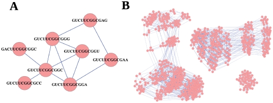
The evolution and adaptation of molecular populations is constrained by the diversity accessible through mutational processes. RNA is a paradigmatic example of biopolymer where genotype (sequence) and phenotype (approximated by the secondary structure fold) are identified in a single molecule. The extreme redundancy of the genotype-phenotype map leads to large ensembles of RNA sequences that fold into the same secondary structure and can be connected through single-point mutations. These ensembles define neutral networks of phenotypes in sequence space. Here we analyze the topological properties of neutral networks formed by 12-nucleotides RNA sequences, obtained through the exhaustive folding of sequence space. A total of 4(12) sequences fragments into 645 subnetworks that correspond to 57 different secondary structures. The topological analysis reveals that each subnetwork is far from being random: it has a degree distribution with a well-defined average and a small dispersion, a high clustering coefficient, and an average shortest path between nodes close to its minimum possible value, i.e. the Hamming distance between sequences. RNA neutral networks are assortative due to the correlation in the composition of neighboring sequences, a feature that together with the symmetries inherent to the folding process explains the existence of communities. Several topological relationships can be analytically derived attending to structural restrictions and generic properties of the folding process. The average degree of these phenotypic networks grows logarithmically with their size, such that abundant phenotypes have the additional advantage of being more robust to mutations. This property prevents fragmentation of neutral networks and thus enhances the navigability of sequence space. In summary, RNA neutral networks show unique topological properties, unknown to other networks previously described.

Figure 1. Construction of neutral networks.

In (A), we show an example of how neutral networks are constructed: sequences that fold into the same secondary structure are connected if they are at a Hamming distance of one. In (B), we show all sequences of length 12 that fold into the secondary structure (.(....))..., which is ranked in the 46th position. Although all sequences fold into the same secondary structure, the neutral network splits into 3 isolated subnetworks of sizes N = 404, 341, and 55.

Figure 2. Subnetworks size ranking.

In linear-logarithmic scale, ranking distribution of subnetwork sizes. Colors indicate the number of base pairs L_p in the secondary structure: one pair (black), two pairs (red), three pairs (green) and four pairs (blue). The solid line corresponds to an exponential fitting. Insets show for each group of structures (with the same L_p) the size of the subnetworks (in the y-axis) that belong to the same neutral network as a function of the corresponding neutral network size (in the x-axis). Note changes of scale in both axes.

Figure 3. Degree distribution p(k) and average degree

(A) Degree distribution p(k) of fifteen subnetworks. They are the five largest (black curves), five of intermediate size (brown curves, one order of magnitude smaller) and five small subnetworks (blue curves, two orders of magnitude smaller). (B) Average degree as a function of the subnetwork size N. Colors correspond to one (black), two (red), three (green) and four (blue) base pairs in the secondary structure. The solid line corresponds to the numerical fitting (note the logarithmic-linear scale). The analytical approximation to making use of the values of , and α obtained from all the 12-nt folded sequences (and implying A_S = 0.53) is plotted in long-dashed black line. The upper and lower bounds to coefficient A_S yield and (plotted in short-dashed red lines).

Figure 4. Clustering.

(A) Clustering distribution C(k) for the fifteen networks analyzed in Fig. 3. (B) Average clustering C(N) as a function of the subnetwork size N for all folded neutral networks (colored circles), equivalent random networks (black squares) and theoretical predictions with a classical random model (, green stars). Circle colors correspond to the number of base pairs of each subnetwork (see caption of Fig. 3). In both plots (A) and (B), the analytical approximations using the values of , and α obtained from all the 12-nt folded sequences are plotted in long-dashed black lines.

Figure 5. Assortativity.

(A) Average nearest neighbors degree k_nn(k) as a function of k for fifteen networks of different sizes. (B) Assortativity parameter r as a function of the network size. As in previous figures, colors correspond to the number of base pairs of the subnetwork: one (black), two (red), three (green) and four (blue). The r for equivalent random networks are plotted in black squares.

Figure 6. Probability of mutation.

Probability of mutation at each position of the sequence for two different secondary structures (see x-axis labels of both plots). (A) corresponds to the largest subnetwork N = 57481, whose secondary structure is fourth by abundance. (B) corresponds to the largest subnetwork N = 35594 of the most abundant secondary structure. We plot the sequences grouped by degree (dotted, dashed and dashed-dotted lines) together with their averages (solid lines).

Figure 7. Average shortest path

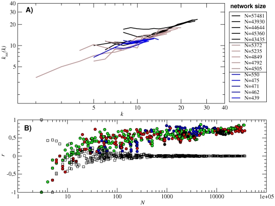
Dependence of the average shortest path on the subnetwork size N for all folded neutral networks (colored circles), equivalent random networks (black squares) and theoretical predictions with a classical random model (, green stars). Circle colors correspond to the number of base pairs of each subnetwork (see caption of Fig. 3). The numerical fitting is plotted as a solid black line, while the analytical approximations correspond to the long-dashed black lines (for values of α and A_S numerically obtained from the folding of all 12-nt sequences). Inset (A): relation between the average shortest path and the average Hamming distance of the subnetworks. Inset (B): relation between the longest distance between any pair of nodes of the network d_max and the maximum number of different bases between sequences H_max (maximum Hamming distance). In the insets, the dashed lines are and , which correspond to the lower bounds of and , respectively.

Figure 8. Eigenvector centrality.

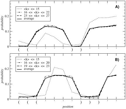
Largest eigenvalue λ ₁ of the adjacency matrix A as a function of the network size N. The inset shows the linear relationship between λ ₁ and the network average degree . Solid line in the inset is .

Figure 9. Sequence centrality.

Evaluation of the sequence centrality for the largest subnetwork N = 57481, whose secondary structure is ((....))..... In (A), degree k_i versus eigenvector centrality v ₁(i). In (B), degree k_i versus betweenness centrality B(i). Colors and shapes denote the type of base pairs the sequences have (see Figure's legend). Note the community division created by the eigenvector centrality, which is related to the type of nucleotides participating in the base pair: GC+UA and AU+CG for low eigenvector centrality, GU+CG and GC+UG and for intermediate v ₁(i) and GC+CG for high v ₁(i).

Figure 10. Comparison between l = 12 and l = 35 neutral networks.

Rank ordering of network sizes for l = 12 (A) and l = 35 (B). Black arrows signal the first non-stem-loop structure. Network size abundance for l = 12 (C) and l = 35 (D). The solid lines correspond to exponential fits, while the dashed line corresponds to a logarithmic decay. Data for l = 35 after .

References

-
- Fontana W, Schuster P. Shaping space: The possible and the attainable in RNA genotypephenotype mapping. J Theor Biol. 1998;194:491–515. - PubMed
- Schuster P. Molecular insights into evolution of phenotypes. In: Crutchfield JP, Schuster P, editors. Evolutionary Dynamics. Oxford Univ. Press; 2003. pp. 163–215.
- Schuster P. Prediction of RNA secondary structures: from theory to models and real molecules. Rep Prog Phys. 2006;69:1419–1477.
- Grüner W, Giegerich R, Strothmann D, Reidys C, Weber J, et al. Analysis of RNA sequence structure maps by exhaustive enumeration. II. Structures of neutral networks and shape space covering. Monatsh Chem. 1996;127:375–389.
- Fontana W, Konings DAM, Stadler PF, Schuster P. Statistics of RNA secondary structures. Biopolymers. 1993;33:1389–1404. - PubMed
Publication types
MeSH terms
Substances
LinkOut - more resources
Full Text Sources