Uncertainty in weather and climate prediction

Abstract

Following Lorenz's seminal work on chaos theory in the 1960s, probabilistic approaches to prediction have come to dominate the science of weather and climate forecasting. This paper gives a perspective on Lorenz's work and how it has influenced the ways in which we seek to represent uncertainty in forecasts on all lead times from hours to decades. It looks at how model uncertainty has been represented in probabilistic prediction systems and considers the challenges posed by a changing climate. Finally, the paper considers how the uncertainty in projections of climate change can be addressed to deliver more reliable and confident assessments that support decision-making on adaptation and mitigation.

Figure 1.

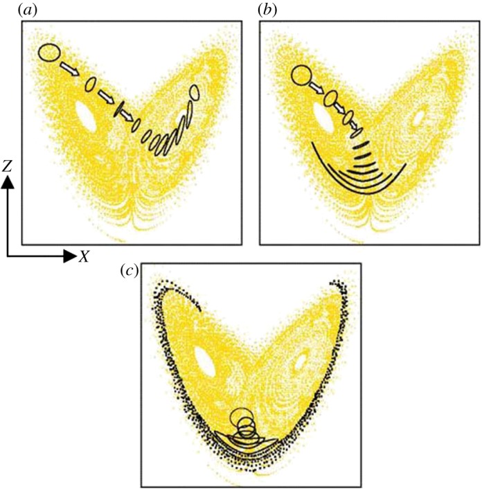
Examples of finite-time error growth on the Lorenz attractor for three probabilistic predictions starting from different points on the attractor. (a) High predictability and therefore a high level of confidence in the transition to a different ‘weather’ regime. (b) A high level of predictability in the near term but then increasing uncertainty later in the forecast with a modest probability of a transition to a different ‘weather’ regime. (c) A forecast starting near the transition point between regimes is highly uncertain.

Figure 2.

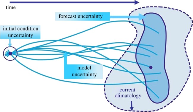
Schematic of a probabilistic weather forecast using initial condition uncertainties. The blue lines show the trajectories of the individual forecasts that diverge from each other owing to uncertainties in the initial conditions and in the representation of sub-gridscale processes in the model. The dashed, lighter blue envelope represents the range of possible states that the real atmosphere could encompass and the solid, dark blue envelope represents the range of states sampled by the model predictions.

Figure 3.

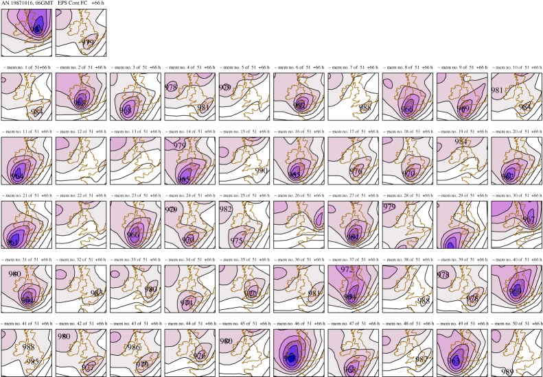
Example of 66 h probabilistic forecast for 15–16 October 1987. Top left shows the analysed deep depression with damaging winds on its southern flank. Top right shows the deterministic forecast, and the remaining 50 panels show other possible outcomes based on perturbations to the initial conditions. A substantial fraction of the ensemble indicates the development of a deep depression.

Figure 4.

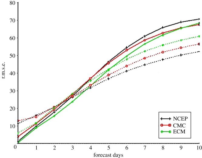
Statistics of ensemble mean forecast error (r.m.s.e.; solid line) and ensemble spread (dotted line) in Northern Hemisphere from three ensemble prediction systems (NCEP, National Center for Environmental Prediction; CMC, Meteorological Service of Canada; ECM, European Centre for Medium-range Weather Forecasting). Note that the forecast error is based on an anomaly forecast and therefore does not include the model systematic bias.

Figure 5.

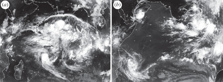
Two infrared satellite images of organized tropical convection over the Indian Ocean for (a) 3 May and (b) 10 May in 2002. The active phase of the Madden–Julian oscillation is centred over the Indian Ocean on 3 May, with many scales of convective organization embedded within it. A week later on 10 May, the Madden–Julian oscillation has propagated eastwards over Indonesia, leaving two tropical cyclones in its wake and an almost clear Indian Ocean. Weather and climate models still have difficulty in capturing the Madden–Julian oscillation and the richness of its structure.

Figure 6.

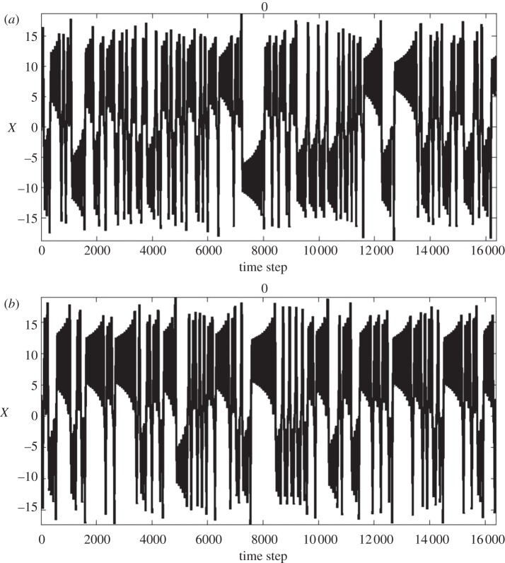
Examples of the time series of the X variable in the Lorenz model, evolving on the Lorenz attractor for (a) no external forcing and for (b) strong external forcing. Changes in probability of the upper regime/lower regime are affected predictably by the imposed ‘forcing’.

Figure 7.

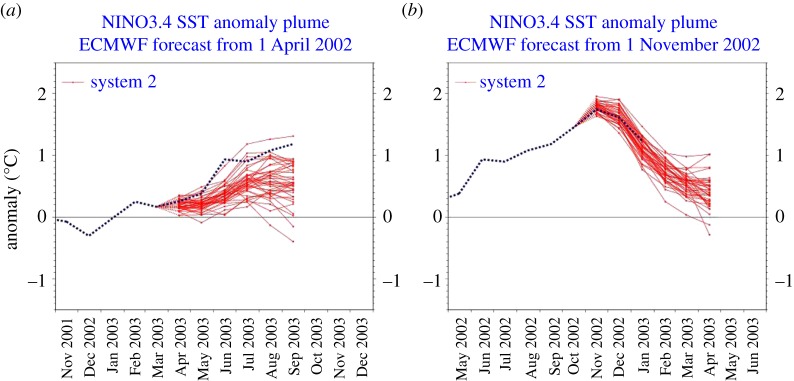
Two contrasting ensemble seasonal forecasts from the European Centre for Medium-range Weather Forecasts (ECMWF) for the evolution of El Nino. (a) The initiation of El Nino is difficult to forecast owing to stochastic forcing from the atmosphere, e.g. westerly wind events. (b) Decay of an El Nino is more predictable owing to the role of equatorial ocean dynamics.

Figure 8.

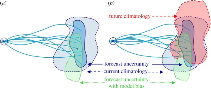
Schematic of ensemble prediction system on seasonal to decadal time scales based on figure 1, showing (a) the impact of model biases and (b) a changing climate. The uncertainty in the model forecasts arises from both initial condition uncertainty and model uncertainty.

Figure 9.

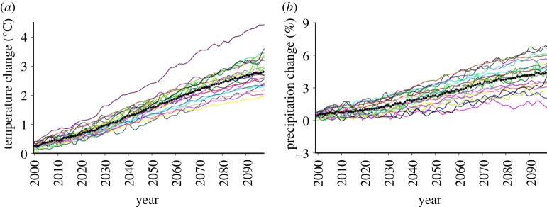
(a) Response of the annual mean surface temperature and (b) precipitation to Special Report on Emission Scenarios A1B emissions, in 21 climate models that contributed to the IPCC Fourth Assessment Report. The solid black line is the multi-model mean.

Figure 10.

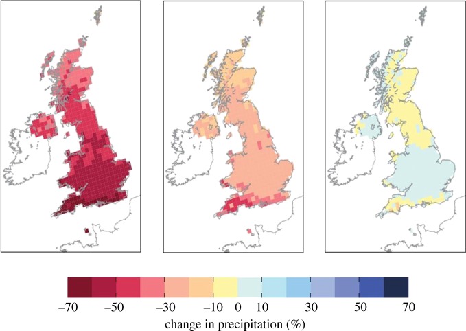
Three potential scenarios of summer rainfall in the 2080s for a high emission scenario (from UKCP09) expressed as a percentage change from the current climate. The middle image shows the central estimate (50% probability) while the left (right) images represent the scenarios where it is unlikely (i.e. 10% probability) that the rainfall may be less (more) than the depicted changes.

Figure 11.

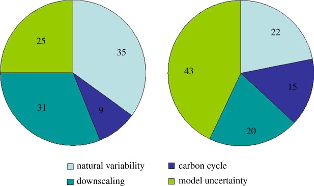
Example of the partitioning of uncertainty in projections of southeast England rainfall for the (a) 2020s and (b) 2080s from UKCP09.

Figure 12.

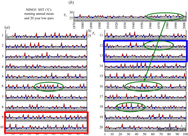
Time series of sea surface temperatures (T_s) for the Nino3 region (5^° S–5^° N and 150^° W–90^° W), in the equatorial east Pacific from (a) 2000 years of climate model simulation with constant forcing representative of the current climate; (b) shows the equivalent time series from observations. Green circles show multi-decadal periods with contrasting El Nino behaviour, including a period in the model's sixteenth century that closely resembles the observed record. Red and blue boxes show extended century-scale periods with contrasting strong and weak El Nino activity, respectively. (Figure courtesy of V. Ramanathan, GFDL, Princeton, NJ, USA).

References

-
- Lorenz E. N. The predictability of a flow which possesses many scales of motion. Tellus. 1969;21:19.
- Lorenz E. N.1963Deterministic nonperiodic flow J. Atmos. Sci. 20130–141. 10.1175/1520-0469(1963)020<0130:DNF>2.0.CO;2 (doi:10.1175/1520-0469(1963)020<0130:DNF>2.0.CO;2) - DOI
- Buizza R., Houtekamer P. L., Pellerin G., Toth Z., Zhu Y., Wei M.2005A comparison of the ECMWF, MSC, and NCEP Global Ensemble Prediction Systems Mon. Wea. Rev. 51076–1097. 10.1175/MWR2905.1 (doi:10.1175/MWR2905.1) - DOI
- Molteni F., Palmer T. N.1993Predictability and finite-time instability of the northern winter circulation Q. J. R. Meteorol. Soc. 119269–298. 10.1002/qj.49711951004 (doi:10.1002/qj.49711951004) - DOI
- Gelaro R., Buizza R., Palmer T. N., Klinker E.1998Sensitivity analysis of forecast errors and the construction of optimal perturbations using singular vectors J. Atmos. Sci. 551012–1037. 10.1175/1520-0469(1998)055<1012:SAOFEA>2.0.CO;2 (doi:10.1175/1520-0469(1998)055<1012:SAOFEA>2.0.CO;2) - DOI
LinkOut - more resources
Full Text Sources