Stability properties of underdominance in finite subdivided populations

Abstract

IN ISOLATED populations underdominance leads to bistable evolutionary dynamics: below a certain mutant allele frequency the wildtype succeeds. Above this point, the potentially underdominant mutant allele fixes. In subdivided populations with gene flow there can be stable states with coexistence of wildtypes and mutants: polymorphism can be maintained because of a migration-selection equilibrium, i.e., selection against rare recent immigrant alleles that tend to be heterozygous. We focus on the stochastic evolutionary dynamics of systems where demographic fluctuations in the coupled populations are the main source of internal noise. We discuss the influence of fitness, migration rate, and the relative sizes of two interacting populations on the mean extinction times of a group of potentially underdominant mutant alleles. We classify realistic initial conditions according to their impact on the stochastic extinction process. Even in small populations, where demographic fluctuations are large, stability properties predicted from deterministic dynamics show remarkable robustness. Fixation of the mutant allele becomes unlikely but the time to its extinction can be long.

Figure 1. Direction of selection in the two population system with migration.

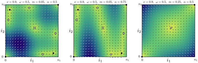
We show a phase portrait of the gradient of selection with . The arrows (length rescaled) indicate the most likely direction of selection given by Eqs. 6–9. The shading indicates the average speed of selection: The darker she shading, the faster the system is expected to leave the given state. Stable fixed points of the replicator dynamics are given by filled disks. Unstable fixed points and saddles are denoted by empty disks. Left panel: The migration rate is below the critical value , such that the replicator dynamics has internal stable fixed points. The number of alleles changes equally fast in both populations . Central panel: For the same migration rate, but with one population changing three times as fast compared to the other (), the selection pattern changes. However, the fixed points of the replicator dynamics Eq. 2 remain the same. Right panel: The stability of the fixed points of the replicator dynamics changes critically with the migration rate . For sufficiently high migration rate, , the system proceeds fast to fixation or loss of the mutant allele.

Figure 2. Stochastic evolution of the mutant allele in two coupled populations.

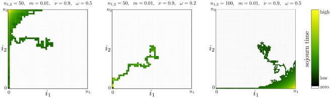
Typical trajectories for the loss of the mutant allele (extinction process) in a system of two populations of the same size, . We show different realizations of the two dimensional Markov chain. The initial condition is the unstable equilibrium near the center , the final state is in all three cases. The shading indicates the sojourn time (total time spent in a particular state, including waiting times). The brighter the shading, the more often the respective state has been visited, white states were not visited. Left panel: Typically, the process spends long times near the corners, where the waiting times are highest. Center panel: The process proceeds fast to extinction of the mutant allele, but slows down near . Right panel: The process spends most of the time in the corner. Once it proceeds to extinction, it moves fast along a boundary of the allele frequency space, i.e. the mutant allele does not invade the other population again.

Figure 3. Fixation becomes unlikely with decreasing fitness of mutant homozygotes, variance in allele frequency increases with migration rate.

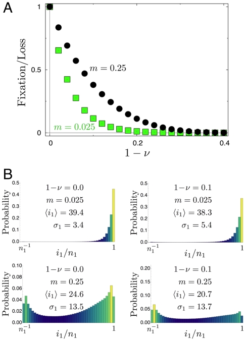
a) The ratio of fixation to loss of the mutant allele in a system of two populations of sizes is shown as a function of the difference of homozygote fitness values , with initial condition , . Results are obtained from independent realizations with a heterozygote fitness of . As approaches , the probability of fixation in both patches goes to zero. b) For four different scenarios of homozygote fitness and migration rate we show the quasi-stationary distribution of the number of mutant alleles in population 1 (, independent realizations with initial conditions ). The average number of mutants in population is denoted by , the standard deviation by . As homozygotes become less fit, the distribution does not change significantly. However, increases with migration rate.

Figure 4. Mutant allele's extinction is delayed for small but non-vanishing migration rates.

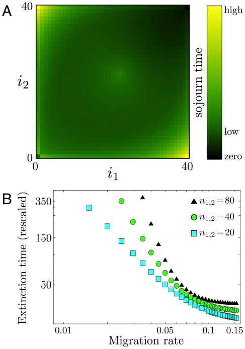
(a) Histogram of the extinction process and the according extinction times as functions of the migration rate in systems of two equally large populations (, , , ). This histogram can be obtained by averaging over sample trajectories such as those shown in Fig. 2. The initial condition is the unstable equilibrium near the center , the outcomes are conditioned on extinction (final state ). Histogram across the entire state space, , ( realizations). For each state we give a record of the time spent. Black states are never visited, colored states are visited at least once. The brighter the color, the more often the respective state has been visited, which is characterized by a sojourn time in that state. (b) The mean extinction time rescaled by , for three different system sizes as a function of , in a double logarithmic plot. Symbols refer to (squares), (circles), (triangles) ( realizations).

Figure 5. Transition from rapid to slow extinction as migration rate decreases.

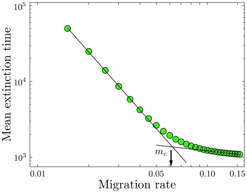
The mean extinction time as a function of the migration rate ( realizations) for , in a double logarithmic plot for mutant homozygote fitness and heterozygote fitness . The initial condition is near the deterministic unstable equilibrium . The arrow indicates the value of critical migration rate of the deterministic replicator dynamics, Eq. 2, . Values for the probability of extinction for the same parameters are () and ().

Figure 6. Maintenance of polymorphism in a small island population.

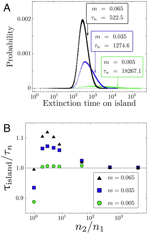
a) Histograms of the extinction time on an island population, Eqs. 12,13, for different migration rates in a log-linear plot. Population size is , fitness of mutant homozygotes is , fitness of heterozygotes is . The histograms stem from independent realizations with initial condition . Each arrow indicates the mean extinction time , Eq. 22 (). The values from simulation and the exact formula are in excellent agreement. With decreasing migration rate, the distribution of extinction times broadens significantly. b) For the same set of parameters we show how the (conditional) average extinction time of the mutant allele in a small population converges to the analytical result of the continent-island approximation with and variable ( independent realizations).

Figure 7. Searching for an optimal release strategy.

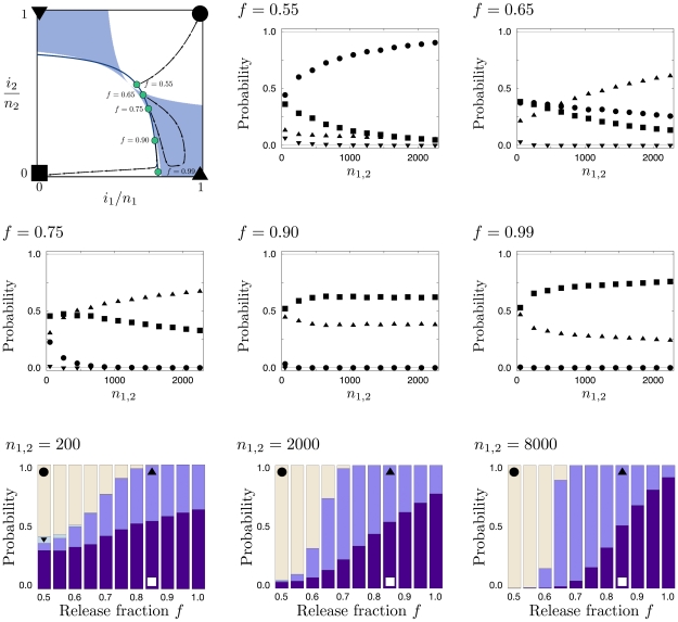
The upper left panel illustrates the deterministic basins of attraction for , , and . The blue line illustrates possible starting points for a release of size for all possible values of the release fraction, , into population 1. Blue disks correspond to points of illustration in the five following panels. The arrow streams represent example trajectories of deterministic dynamics. The following five panels are labeled according to the release fraction . Symbols correspond to the probability of reaching the correspondingly labeled corners (in the upper left panel) and indicate how they change with . Although complete fixation or loss are the only possible long term events, there is a probability that the neighborhood of, e.g., , is reached first, which we refer to here by triangles. In particular, note that the probability ranks interchange at certain population size for and . The three bottom panels, labeled with the respective system sizes, show the corner probabilities as a function of . A release strategy with maximizes the likelihood of transforming both populations. In contrast to that, , maximizes the likelihood of transforming only a target local population. Higher values of then proceed to an increasing likelihood of rapid loss in both populations. All results are obtained from independent realizations.

References

-
- Fisher RA. On the dominance ratio. Proc Roy Soc Edinburgh. 1922;42:321–341.
- Haldane JBS. A mathematical theory of natural and artificial selection. Part V. Selection and mutation. Proc Camb Philol Soc. 1927;23:838–844.
- Hartl DL, Clark AG. Principles of Population Genetics. 3rd edition. Sunderland, MA: Sinauer Associates, Inc; 1997.
- Li CC. The stability of an equilibrium and the average fitness of a population. Am Nat. 1955;89:281–295.
Publication types
MeSH terms
LinkOut - more resources
Full Text Sources
Other Literature Sources