Identification of cortical lamination in awake monkeys by high resolution magnetic resonance imaging

Abstract

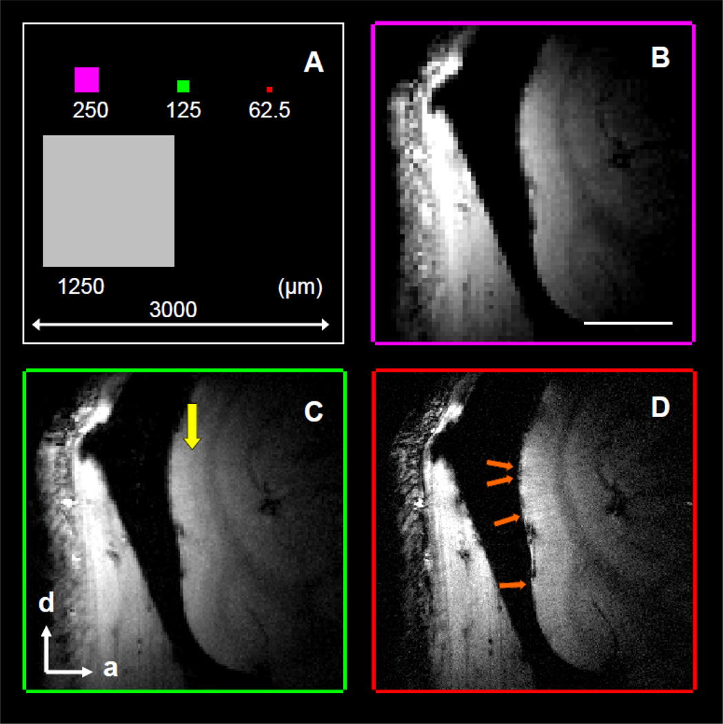
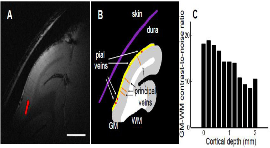
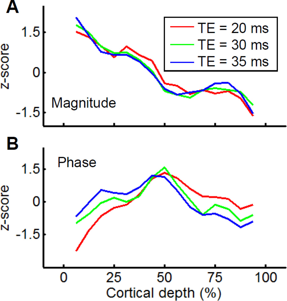
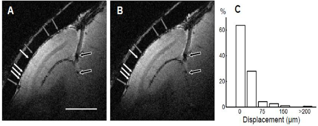
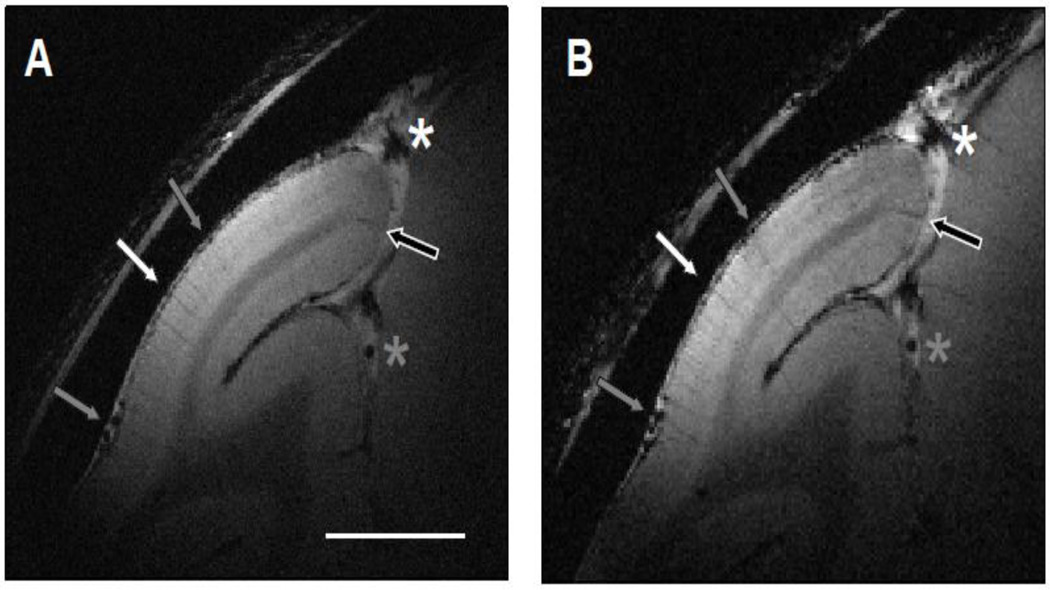
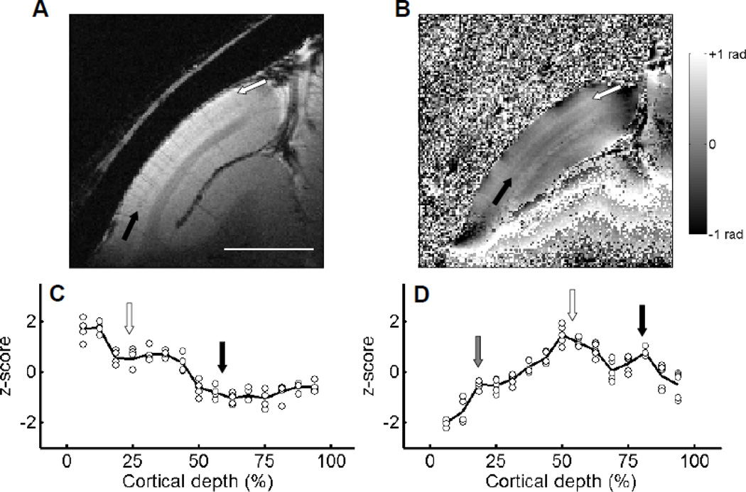
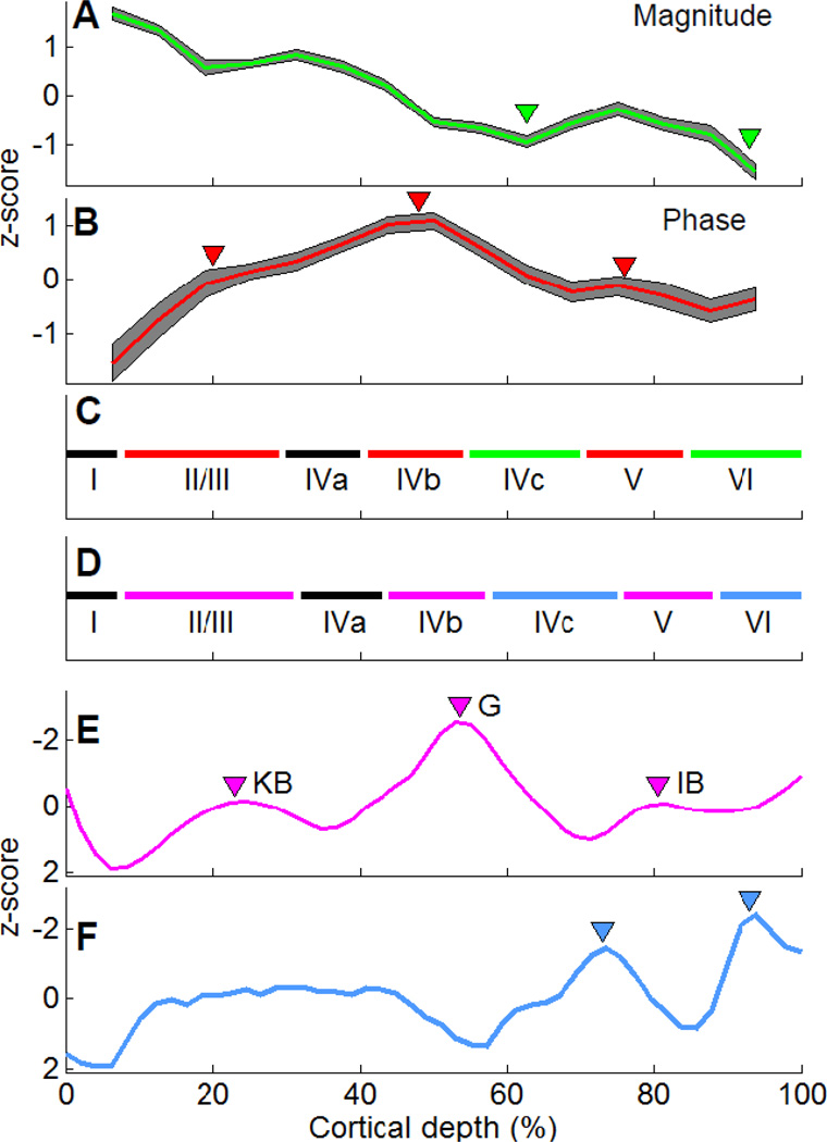
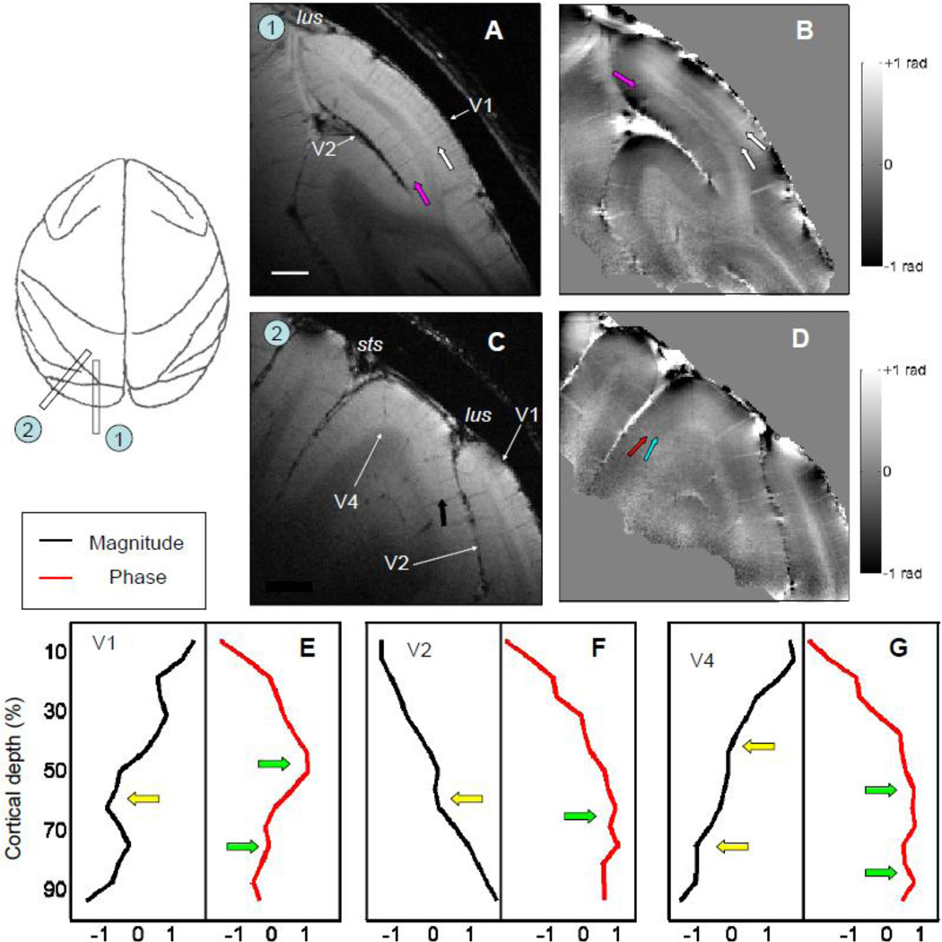
Brodmann divided the neocortex into 47 different cortical areas based on histological differences in laminar myeloarchitectonic and cytoarchitectonic defined structure. The ability to do so in vivo with anatomical magnetic resonance (MR) methods in awake subjects would be extremely advantageous for many functional studies. However, due to the limitations of spatial resolution and contrast, this has been difficult to achieve in awake subjects. Here, we report that by using a combination of MR microscopy and novel contrast effects, cortical layers can be delineated in the visual cortex of awake subjects (nonhuman primates) at 4.7 T. We obtained data from 30-min acquisitions at voxel size of 62.5 × 62.5 × 1000 μm(3) (4 nl). Both the phase and magnitude components of the T(2)*-weighted image were used to generate laminar profiles which are believed to reflect variations in myelin and local cell density content across cortical depth. Based on this, we were able to identify six layers characteristic of the striate cortex (V1). These were the stripe of Kaes-Bechterew (in layer II/III), the stripe of Gennari (in layer IV), the inner band of Baillarger (in layer V), as well as three sub-layers within layer IV (IVa, IVb, and IVc). Furthermore, we found that the laminar structure of two extrastriate visual cortex (V2, V4) can also be detected. Following the tradition of Brodmann, this significant improvement in cortical laminar visualization should make it possible to discriminate cortical regions in awake subjects corresponding to differences in myeloarchitecture and cytoarchitecture.

Figure 1. Influence of in-plane resolution on image quality

(A) The relative in-plane size of voxels used in this and other MR imaging studies. (B–D) The T₂*-weighted images (slice thickness 2 mm) from the visual cortex of an awake monkey as a function of in-plane resolution. The in-plane resolutions are 250 × 250 µ², 125 × 125 µm², and 62.5 × 62.5 µm² for (B), (C), and (D), respectively. The stripe of Gennari (yellow arrow in C) and cortical veins (orange arrows in D) are detectable. Scale bar in (B): 5 mm. d, dorsal; a, anterior.

Figure 2. High-resolution structural image in the awake monkey V1

(A) A high-resolution structural image with in-plane resolution of 62.5 × 62.5 µm² and slice thickness of 1 mm shows fine anatomical structures of V1. The slice is oriented perpendicular to the cortical surface. The gray and white matter are clearly separable, and the stripe of Gennari (red arrow) can be seen in the middle of gray matter. (B) Illustration of anatomical structures. Skin and dura are marked as purple and yellow lines, respectively. Pial veins are indicated by red dots, and principal veins running through the gray matter are shown as orange lines. WM, white matter. GM, gray matter. Scale bar in (A): 5 mm. (C) The contrast-to-noise ratio between the gray matter and white matter plotted against the cortical depth.

Figure 3. Cortical depth profiles of T₂* weighted images are a function of echo time (TE)

The magnitude (A) and the phase (B) profiles of T₂* weighted images. The average profiles at different echo time of 20 ms, 30 ms, and 35 ms are marked as red, green, and blue lines. Profiles are z-normalized and plotted against the distance from the cortical surface in percent of cortical depth for a better comparison.

Figure 4. Reproducibility of structural images within a session

(A and B) Structural images collected in two runs (30 minutes each) that were one hour apart (slice thickness, 1 mm; in-plane resolution, 100 × 100 µm²). The locations of the pial veins (black and gray arrows) and principal veins within gray matter (white arrows) are the same. Scale bar: 5 mm. (C) The distribution of relative displacement between runs in the duration of 30 minutes (the length of a typical run).

Figure 5. Reproducibility of structural images between sessions

Structural images of V1 from the same awake monkey collected in two sessions that were 2 weeks apart are shown. (A) The in-plane voxel size was 62.5 × 62.5 µm² and the thickness was 1 mm. (B) In-plane spatial resolution of 100 × 100 µm² and a thickness of 1 mm. The location and shape of the pial veins within the lunate sulcus (white and gray stars) and on the cortical surface (gray arrows) are almost the same. The repeatable detection of principal veins within gray matter (gray and white arrows) further support that the high-resolution structural images from different sessions are highly reproducible. Scale bar: 5 mm.

Figure 6. Cortical profiles of magnitude and phase in V1

The magnitude (A) and phase (B) images of averaged results from five 30-minute runs of a slice over V1 (slice thickness, 1 mm; in-plane resolution, 100 × 100 µm²). The stripe of Gennari (black arrow, layer IV) can be detected in (A). An additional dark layer can be found between the cortical surface and the layer IV (white arrow) from the magnitude map (A). From the phase map (B), a second bright layer (black arrow) exists between the layer IV (white arrow) and the white/gray matter border. (C) and (D) show the z-normalized profiles of magnitude and phase against cortical depth. The black lines indicate the averaged results, and circles represent results of individual runs. Locations of prominent laminar structures are indicated by arrows with the same color used in (A) and (B). A small third peak at 20% cortical depth can be detected in the phase profile (gray arrow). Scale bar in (A): 5 mm.

Figure 7. Results from high resolution MRI reflect the myeloarchitecture and the cytoarchitecture of V1

The averaged results of magnitude (A) with dips marked (green triangles) from all runs and slices. The averaged results of phase profiles (B) with peaks marked (red triangles). The gray shadings represent the 95% confidence level in (A) and (B). (C) The laminar structure determined by MRI with peaks in phase profile (red lines) and dips in magnitude profile (green lines) marked. The laminar structure determined by conventional histology is shown in (D). Cell (E) and myelin densities (F) of V1 from literature are z-normalized and plotted against cortical depth with cortical areas of high myelin density marked by pink triangles and regions with high cell density marked by blue triangles. KB: the stripe of Kaes-Bechterew. G: the stripe of Gennari. IB: the inner band of Baillarger. The direction of y-axis of (D) and (E) is reversed for comparison.

Figure 8. MR structural images of extrastriate visual cortex

The magnitude (A) and phase (B) images of a parasagittal slice revealed V2 buried in the lunate sulcus (lus). Besides the stripe of Gennari (white arrow) in V1, a dark layer (pink arrow) can be found in the middle of V2 from the magnitude map (A). From the phase map (B), one bright layer exists in V2 (pink arrow) in additional to the two bright layers in V1 (white arrows). (C) and (D) An oblique slice that includes the portion of V4 that located between superior temporal sulcus (sts) and lus. Laminar structures within V4 (black arrows) can be found both from magnitude map (C) and phase map (D). The averaged results of magnitude (black lines) and phase profiles (red lines) from prestriate visual cortex of V1 (E), V2 (F), and V4 (G) are summarized. The peaks in phase profiles and dips in magnitude profiles are marked by green and yellow arrows, respectively. Both images were acquired with in-plane voxel size of 100 × 100 µm², thickness of 1 mm, and flip angle of 45°. Scale bar: 2 mm in (A).

References

1. Abduljalil AM, Schmalbrock P, Novak V, Chakeres DW. Enhanced gray and white matter contrast of phase susceptibility-weighted images in ultra-high-field magnetic resonance imaging. J Magn Reson Imaging. 2003;18:284–290. - PubMed
1. Baillarger JGF. Recherches sur la structure de la couche corticale des circonvolutions du cerveau. Mem. Acad. R. Med. 1840;8:149–183.
1. Barbier EL, Marrett S, Danek A, Vortmeyer A, van Gelderen P, Duyn J, Bandettini P, Grafman J, Koretsky AP. Imaging cortical anatomy by high-resolution MR at 3.0T: detection of the stripe of Gennari in visual area 17. Magn Reson Med. 2002;48:735–738. - PubMed
1. Bechterew W. Zur Frage uber die ausseren Associationsfasern der Hirnrinde. Neurol Zentrbl. 1891;10:682–684.
1. Benveniste H, Blackband S. MR microscopy and high resolution small animal MRI: applications in neuroscience research. Prog Neurobiol. 2002;67:393–420. - PubMed
Publication types