Iterative Bayesian estimation as an explanation for range and regression effects: a study on human path integration

Abstract

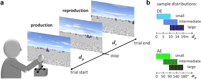
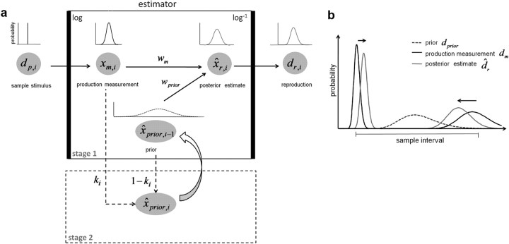
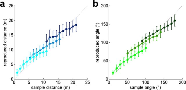
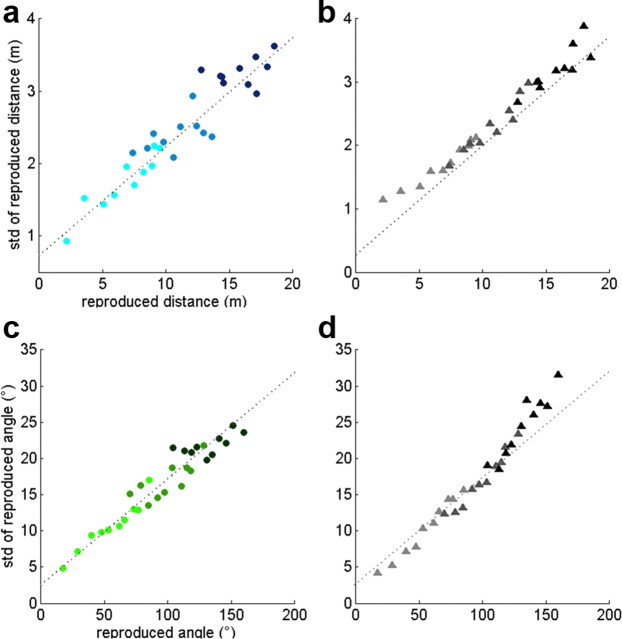
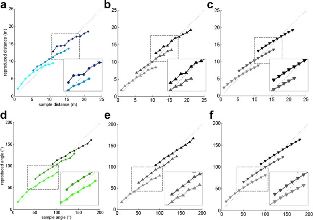
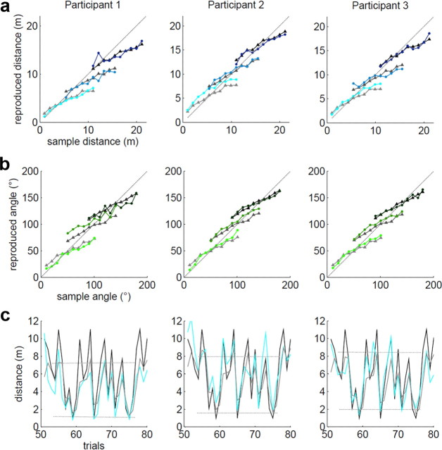
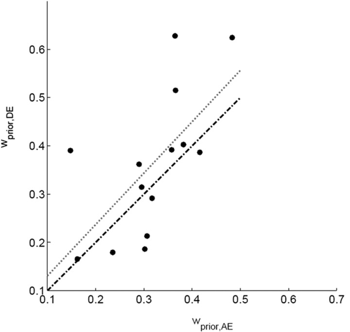
Systematic errors in human path integration were previously associated with processing deficits in the integration of space and time. In the present work, we hypothesized that these errors are de facto the result of a system that aims to optimize its performance by incorporating knowledge about prior experience into the current estimate of displacement. We tested human linear and angular displacement estimation behavior in a production-reproduction task under three different prior experience conditions where samples were drawn from different overlapping sample distributions. We found that (1) behavior was biased toward the center of the underlying sample distribution, (2) the amount of bias increased with increasing sample range, and (3) the standard deviation for all conditions was linearly dependent on the mean reproduced displacements. We propose a model of bayesian estimation on logarithmic scales that explains the observed behavior by optimal fusion of an experience-dependent prior expectation with the current noisy displacement measurement. The iterative update of prior experience is modeled by the formulation of a discrete Kalman filter. The model provides a direct link between Weber-Fechner and Stevens' power law, providing a mechanistic explanation for universal psychophysical effects in human magnitude estimation such as the regression to the mean and the range effect.

Figure 1.

The production–reproduction task. a, Temporal sequence of events in each test trial. Participants had to produce and subsequently reproduce a certain displacement in the VR by using the joystick. Depending on the session, participants walked on a linear path (DE) or turned on the spot (AE) until they were automatically stopped after a certain displacement, d_p or α_p, respectively. Next, participants were instructed to reproduce the same amount of perceived displacement while keeping the direction of movement constant. Participants indicated that they reached their final position by a button press. This estimated displacement is referred to as d_r in DE sessions and α_r in AE sessions. b, DE and AE were tested separately under three different conditions that differed only in the underlying uniform sample distribution (small displacements, intermediate displacements, and large displacements range, for DE: turquoise, light blue, and dark blue, respectively; for AE: bright green, olive, dark green, respectively) from which the production displacements d_p and α_p were drawn.

Figure 2.

Two-stage Bayesian estimator model on logarithmic scales. a, Schematic estimation process. Stage 1, The produced displacement d_p,i in trial i is represented by the Bayesian estimator as a measurement likelihood on logarithmic scales p(x_m,i). The posterior estimate of displacement is determined by the weighted average of the measurement x_m,i and an a priori estimate of displacement x̂_prior,i−1, with weights of measurement w_m and prior w_prior, resulting after backtransform in a reproduced displacement on linear scales d_r,i. Stage 2, The posterior estimate of the prior in trial i, x̂_prior,i, is estimated before the next trial according to the weighted average of the a priori estimate x̂_prior,i−1 and the measurement x_m,i, with weights k_i and 1 − k_i, modeled by the discrete formulation of the Kalman filter, where k_i refers to the Kalman gain. The posterior is updated over time to build the prior estimate x̂_prior,i−1 in the subsequent trial. b, Example for the effect of the Bayesian estimator model on linear scales for a particular sample interval. If the prior d_prior is close to the mean of the sample interval, Bayesian fusion with the measurement d_m leads to a posterior estimate d_r that overestimates small displacements and underestimates large displacements. The effect is stronger for larger displacements (black arrows), due to the calculation of the weighted average on logarithmic scales and thus an increased standard deviation with increasing mean on linear scales.

Figure 3.

Mean displacement estimation behavior over all participants for the three prior experience conditions (small displacements, intermediate displacements, and large displacements range). a, Mean participants' response in DE sessions in virtual meters (blues). b, Mean participants' response in AE sessions in degrees (greens). Error bars depict the standard deviation between participants' responses. The dotted line indicates were the response and sample stimulus would be equal. In both experiments, the behavior deviated significantly from the line of equality depending on the prior experience condition. Small displacements were underestimated and large displacements were overestimated in all conditions. The bias increased for increasing sample range, being strongest for the large displacements range (dark colors). Small displacements, intermediate displacements, and large displacements range, for DE: turquoise, light blue, and dark blue, respectively; for AE: bright green, olive, dark green, respectively.

Figure 4.

Mean predicted and actual reproduced displacement estimation and corresponding mean standard deviation (std). a, Experimental DE data of mean participants' responses for all three conditions (blue dots) and linear regression (dotted line). b, Two-stage model prediction for DE data (triangles) and same regression (dotted line) as in a for comparison with the experimental data. c, Experimental AE data of mean participants' responses for all conditions (green dots) and linear regression (dotted line). d, Two-stage model predictions for AE sessions and same regression line as in c for comparison with the experimental data. Small displacements, intermediate displacements, and large displacements range, for DE: turquoise, light blue, and dark blue, respectively; for AE: bright green, olive, dark green, respectively.

Figure 5.

Summary of predicted and actual displacement estimation behavior. a, d, Mean reproduced distances in DE (a, blue dots) and AE (d, green dots) sessions for all conditions (small displacements, intermediate displacements, and large displacements range, for DE: turquoise, light blue, and dark blue, respectively; for AE: bright green, olive, dark green, respectively). b, e, Corresponding prediction of the fitted two-stage model (upward gray triangles). c, f, Corresponding prediction of the fitted one-stage model (downward gray triangles). The dotted lines in all plots indicate were reproduced estimate and sample displacement would be equal. Insets show small variations in the participants' responses that are captured by the two-stage model with varying prior but not by the one-stage model with fixed prior.

Figure 6.

Comparison of individual participants' responses with predicted behavior of the two-stage model. a, Mean responses of three selected participants in DE sessions and model predictions (gray triangles, w_{prior,Participant1} = 0.39, w_{prior,Participant2} = 0.39, w_{prior,Participant3} = 0.40). b, Mean responses of the same participants in AE sessions and model predictions (gray triangles, w_{prior,Participant1} = 0.15, w_{prior,Participant2} = 0.36, w_{prior,Participant3} = 0.38). c, Example of a typical time course for the same participants of sample displacements (black line), reproduced displacements (light blue line), and predicted displacements (gray line) within 30 trials of one DE session (small displacements range, trials: 50–80). Dotted lines indicate the range of displacements covered by the prediction of the model. Small displacements, intermediate displacements, and large displacements range, for DE: turquoise, light blue, and dark blue, respectively; for AE: bright green, olive, dark green, respectively.

Figure 7.

Comparison of the weighting of the prior within participants. Each dot represents the weight w_prior in AE and DE sessions for one participant. The gray dotted line indicates the linear regression between the two weights and the black dotted line is the line of equality.

References

1. Adams WJ, Graf EW, Ernst MO. Experience can change the ‘light-from-above’ prior. Nat Neurosci. 2004;7:1057–1058. - PubMed
1. Bergmann J, Krauss E, Münch A, Jungmann R, Oberfeld D, Hecht H. Locomotor and verbal distance judgments in action and vista space. Exp Brain Res. 2011;210:13–23. - PubMed
1. Berniker M, Voss M, Körding K. Learning priors for Bayesian computations in the nervous system. PLoS One. 2010;5:e12686. - PMC - PubMed
1. Burge J, Ernst MO, Banks MS. The statistical determinants of adaptation rate in human reaching. J Vis. 2008;8:20.1–20.19. - PMC - PubMed
1. Butler JS, Smith ST, Campos JL, Bülthoff HH. Bayesian integration of visual and vestibular signals for heading. J Vis. 2010;10:23. - PubMed
Publication types
LinkOut - more resources