Self-organizing circuit assembly through spatiotemporally coordinated neuronal migration within geometric constraints

Abstract

Background: Neurons are dynamically coupled with each other through neurite-mediated adhesion during development. Understanding the collective behavior of neurons in circuits is important for understanding neural development. While a number of genetic and activity-dependent factors regulating neuronal migration have been discovered on single cell level, systematic study of collective neuronal migration has been lacking. Various biological systems are shown to be self-organized, and it is not known if neural circuit assembly is self-organized. Besides, many of the molecular factors take effect through spatial patterns, and coupled biological systems exhibit emergent property in response to geometric constraints. How geometric constraints of the patterns regulate neuronal migration and circuit assembly of neurons within the patterns remains unexplored.

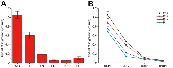
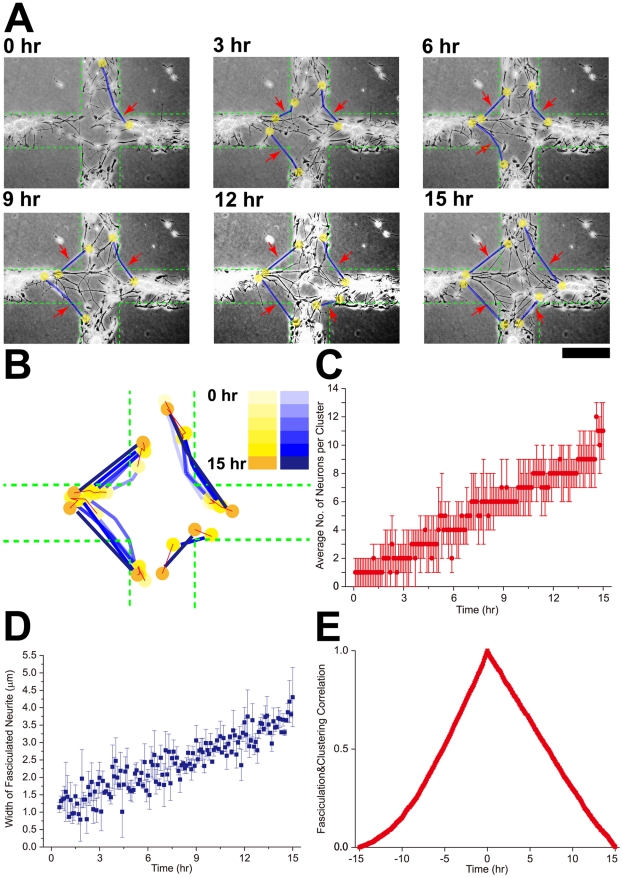
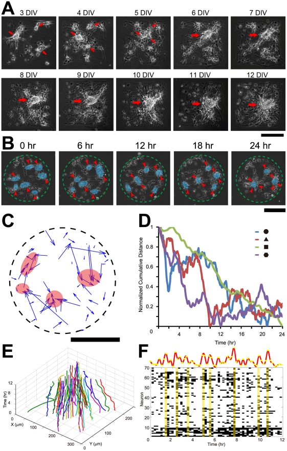
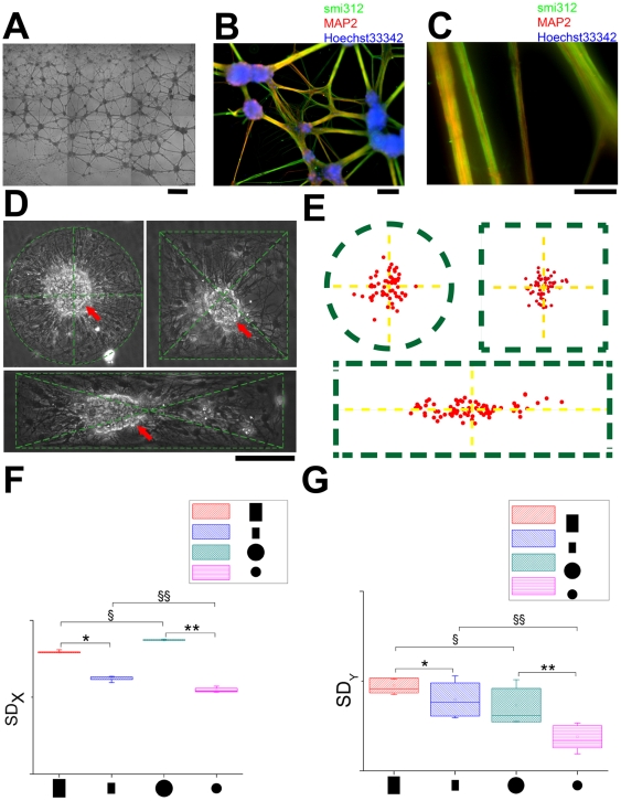
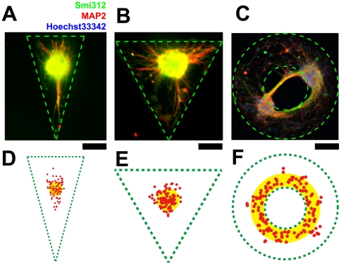
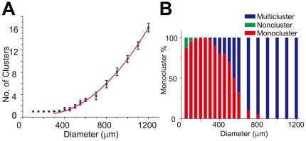
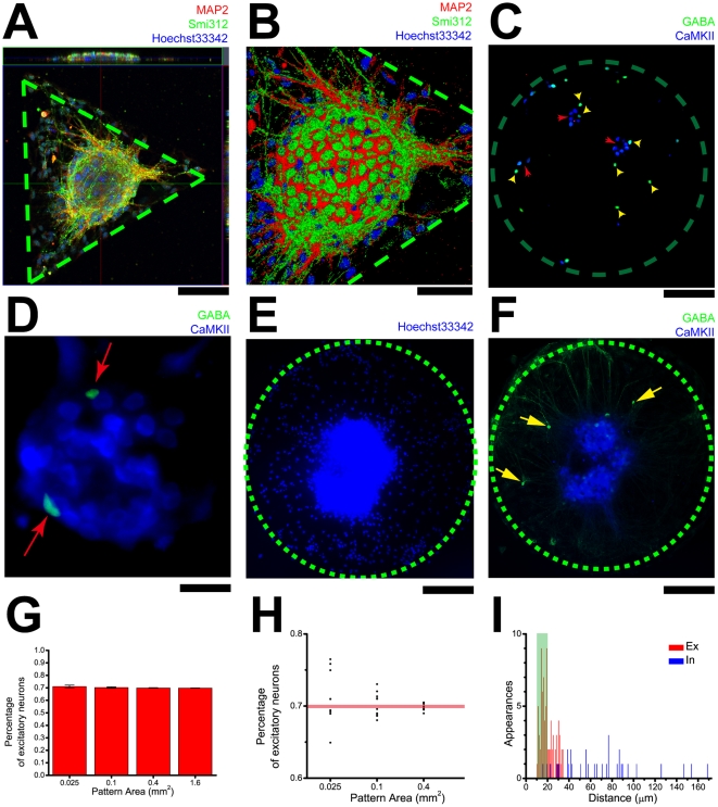
Methodology/principal findings: We established a two-dimensional model for studying collective neuronal migration of a circuit, with hippocampal neurons from embryonic rats on Matrigel-coated self-assembled monolayers (SAMs). When the neural circuit is subject to geometric constraints of a critical scale, we found that the collective behavior of neuronal migration is spatiotemporally coordinated. Neuronal somata that are evenly distributed upon adhesion tend to aggregate at the geometric center of the circuit, forming mono-clusters. Clustering formation is geometry-dependent, within a critical scale from 200 µm to approximately 500 µm. Finally, somata clustering is neuron-type specific, and glutamatergic and GABAergic neurons tend to aggregate homo-philically.

Conclusions/significance: We demonstrate self-organization of neural circuits in response to geometric constraints through spatiotemporally coordinated neuronal migration, possibly via mechanical coupling. We found that such collective neuronal migration leads to somata clustering, and mono-cluster appears when the geometric constraints fall within a critical scale. The discovery of geometry-dependent collective neuronal migration and the formation of somata clustering in vitro shed light on neural development in vivo.

Figure 1. Surface coating and developmental stage modulates the speed of neuronal migration on gold substrate.

A, The speed of migration of neurons from E16 rat pups at 0 DIV, cultured on MG coated gold surfaces is significantly higher than those on other surfaces. (MG: n = 24, LN: n = 20, FN: n = 20, PDL: n = 20, PLL: n = 18, PEI: n = 8. P<0.01. One way ANOVA followed by Tukey's post hoc test, see Figure S1 for details). The speed of migration is determined by time-lapse imaging at a rate of 10 seconds per frame and calculating the speed by dividing the displacement by the time interval. Note that the long term displacement is zero for any surface coating other than MG and LN (refer to the Materials and Methods section for details). B, The speed of migration of neurons at different developmental stages. The speed of migration decreases against the age of the donor animals and the culture. (E16: n = 5, 30 data points at each time; E18: n = 8, 30 data points at each time; E19: n = 8, 30 data points at each time; P1: n = 8, 30 data points at each time. Spearman's rho test was used for monotonicity between speed of migration and age of culture, correlation coefficients are E16: 0.77856, P<0.001; E18: 0.70401, P<0.001; E19: 0.70456, P<0.001; P1: 0.80623, P<0.001. Mann- Kendall's tau test for monotonicity between speed of migration and age of donor animal (P1 treated as E23), correlation coefficients are 0DIV: 0.40882, P<0.001; 2DIV: 0.30561, P<0.001; 6DIV: 0.22818, P<0.001; 12DIV: 0.31062, P<0.001.) Error bars denote S.E.M.

Figure 2. Correlated neurite fasciculation and somata migration.

A, Time lapse imaging showing the emergence and evolution of fasciculated neurites (highlighted by light blue lines) accompanied by somata (highlighted by yellow balls) migration over 15 hrs at 3DIV. The geometric constraint was specifically designed so that neuronal somata could only migrate along the area of the cross-shaped geometric constraint (confined to the green dashes) while neurites connecting clusters are not limited by the geometric constraint. B, Color-coded superimposed silhouettes of fasciculated neurites and somata clusters from panel A illustrates the relationship between fasciculation and clustering. A series of blue colors represent the neurites while yellow shades represent the clusters, the depth of color grows as time elapses. Red solid lines represent the migratory trajectory of the cluster and green dashes show the edges of the geometric constraint. C, The average number of neurons within a cluster grows (from 1±1 to 11±2 during the 15 hrs time window, n = 5, 20 data points for each time point) as time elapses, indicating time-evolved recruitment of neurons. D, The width of the fasciculated neurites grows (from 0.91047±0.1003 µm to 4.30173±0.84857 µm, n = 5, 20 data points for each time point) over time. E, Correlation between the number of neurons (Figure 2C) and the width of neurites (Figure 2D). The horizontal axis represents the temporal shift between the two variables, and the highest value is achieved with no time shift, meaning these two events are temporally correlated. Scale bar: 200 µm.

Figure 3. Collective dynamics of neuronal migration within geometric constraints is spatiotemporally coordinated.

A, Time-lapse imaging of a circuit maintained over 12 DIV. The red arrows indicate clusters. As shown here, the clusters gradually come together and finally merge into a mono-cluster. B, Collective neuronal migration over 24 hrs on a circular SAMs geometric constraint (depicted by green dashes) at 2 DIV. Transparent blue shades highlight the clustered somata that are coordinated in migration, red arrows designate the orientation of the migrating clusters. As time elapses, smaller clusters merge into larger ones and gradually approach the geometric center of the geometric constraint. C, The behavior of migration of all 36 neurons (at a lower density) on a circle (black dashes) over 24 hrs at 2 DIV at an interval of 5 min. The blue arrow begins from the original position of the cells at 0 hr, and ends at the final location at 24 hr. Neurons that were evenly distributed throughout the geometric constraint at the beginning finally migrate into a few clusters (transparent pink shades) in the end. D, Cumulative distance curves of all neurons on geometric constraints of different shapes (circular, triangular, square and hexagonal) over 24 hrs at 2 DIV at an interval of 5 min (see Materials and Methods for details on the definition of the curve). E, Collective pattern of neuronal migration on a square-shaped constraint over 12 hrs at 4 DIV at an interval of 5 min. The X-Y axes indicate the spatial locations of all neurons at a specific time, which is represented by the vertical axis. A trace of a particular color corresponds to one neuron. F, The migratory speed of neurons on a square-shaped constraint over 12 hrs at 4 DIV at an interval of 5 min as in panel E is temporally coordinated (P<0.001, Pearson's χ² test, compared with the temporally shuffled random data, see Materials and Methods for details on data analysis). Each black block represents the speed of the specific neuron (indexed by the vertical axis of the block) at a specific time when the speed of migration (indexed by the horizontal axis of the block) is high (above 30%). The vertical axis is the serial number of neurons. The yellow shades highlight time points when most of neurons are migrating at a higher speed. The red curve above is the histogram of the raster plot, showing the number of neurons migrating at a higher speed at each time. The yellow dots represent the number of neurons migrating at high speed at each time point. Scale bars: 200 µm.

Figure 4. Emergence and centrality of mono-cluster on critically-scaled geometric constraints.

A, Phase-contrast photomicrograph of live neurons cultured without geometric constraints at 21 DIV. Individually plated neurons have assembled into randomly located clusters joined through fasciculated neurites. B, Immunocytochemistry showing highly clustered neuronal networks connected by thick and tight fasciculated neurites in panel A. Smi312 is the specific marker of axons, while MAP2 is the specific marker of dendrites. Nuclei are counterstained with Hoechst33342. C, Fasciculated neurites in panel B under higher magnification, the neurites are composed of both axons and dendrites. D, Phase-contrast image of circular, square and rectangular geometric constraints and the deviation of the cluster from the geometric center. Clusters tend to be located in the center on isotropic geometric constraints but retain a degree of freedom on anisotropic geometric constraints like the rectangular geometric constraints. E, Locations of the centers of the clusters on circular, square and rectangular geometric constraints (same as those in panel D) as depicted by the green dashes. The mean radial displacements of the centers of the clusters from the geometric centers are 8±4 µm (circle) 9±6 µm (square) and 32±9 µm (rectangle). The centers are located approximately on the geometric center of the geometry on circular and square constraints and along the central axis parallel to the longer edge on rectangular constraints. (Circular geometric constraint: n = 5, 60 data points; square geometric constraint: n = 5, 60 data points; rectangular geometric constraint: n = 5, 80 data points. The figure is of the same scale as panel D.) F - G, Centrality analysis of circular and rectangular arrays (see Figure S4 for the original image and data extraction procedure). The mean displacements for different shapes are: large rectangles, X = 53±12 µm, Y = 80±34 µm; small rectangle, X = 31±8 µm, Y = 58±29 µm; large circle, X = 65±23 µm, Y = 69±25 µm; small circle, X = 41±11 µm, Y = 38±9 µm. The figures show the box chart of standard deviation of X (upper) and Y (lower) positions among different geometric constraints (SD_X and SD_Y represents standard deviation in x and y directions, respectively. SD_X: *, n = 8, P<0.001. **, n = 8, P<0.001. §, n = 8, P<0.001. §§,n = 8, P<0.001. SD_Y : *, n = 8, 0.01<P<0.1. **, n = 8, P<0.001. §, n = 8, 0.01<P<0.1. §§,n = 8, P<0.001. One-way ANOVA followed by Tukey-Kramer's post-hoc multiple comparisons test). Scale bars: A, 300 µm; B, 100 µm; C, 50 µm; D: 200 µm.

Figure 5. Geometric regulation of clustering location.

A - C, Immunocytochemistry with Smi312 and MAP2 showing cluster location within polarized geometric constraints (A: isosceles triangle, B: equilateral triangle, C: concentric ring). D - F, Locations of the centers of the clusters (red dots) within isosceles triangles, equilateral triangles and concentric rings (corresponding to those in panel A - C, with the same scale) as depicted by the green dashes. The mean radial displacements of the centers of the clusters from the geometric centers are 12±6 µm (isosceles triangle) and 11±7 µm (equilateral triangle). The clusters on the concentric rings are located around the inner radius. The clusters are located around the geometric center (yellow shades) of the shapes (isosceles triangle: n = 5, 90 data points; equilateral triangle: n = 6, 90 data points; concentric ring: n = 8, 120 data points). Scale bars: 200 µm.

Figure 6. The emergence and centrality of mono-cluster is dependent on the size of geometric constraints.

A, The relationship between diameter of the geometric constraint and the number of clusters, red curve is the power law fit (exponent = 2, R = 0.9987, blue error bars denote S.E.M. n = 5, 15–20 data points for each size of geometric constraint.). See Figure S6 for the original data points. B, The percentage (probability) of the appearance of mono-clusters (red) varies with the diameter of the geometric constraint. The highest probability occurs when the diameter of the circular geometric constraint is either 250 or 300 µm. Note that for small geometric constraints there is sometimes no clusters (green) at all, while for large geometric constraints there are multiple clusters (blue). The same set of data as Figure 6A is used.

Figure 7. Location and relative number of excitatory and inhibitory neurons within a network.

A, A clustered network on a triangle with vertical and horizontal sections. Neuronal dendrites are labeled with MAP2 while axons with Smi312, cell nuclei counterstained with Hoechst 33342. B, Higher magnification of the highlighted cluster in a. Somata are assembled into a ball. C, Immunocytochemistry shows that excitatory neurons tend to cluster more than inhibitory neurons do. Excitatory neurons are labeled with CaMKII while inhibitory neurons are labeled with GABA (refer to the text for details). D, Higher magnification of a cluster. Inhibitory neurons labeled by GABA locate in the periphery of the cluster that is primarily composed of excitatory neurons. E, The location of all cell nuclei within a network. F, The location of excitatory and inhibitory neurons on the same network as E, while most of the neuron somata are clustered in the center of the network, a few somata of inhibitory neurons only are scattered in the periphery of the network. G, The percentage of excitatory neurons in the overall population on geometric constraints of different sizes. Note that there is substantial fluctuation of the total number of neurons among geometric constraints. As the area grows, the ratio gradually approaches unrestrained cultures with large number of cells. (n = 5, 10–15 data points for each size of geometric constraint.) H, Scatterogram showing the distribution of the ratio on geometric constraints of various areas. As the area increases, less fluctuation is present in the percentage. The same set of data as panel G is used. I, Histogram showing that inhibitory neurons tend to stay away from the clusters, indicating a heterogeneous nature in neuronal migration and cluster formation. The green shade represents the range where the diameters of neurons generally fall within. (n = 5, 42 excitatory neurons, 21 inhibitory neurons.) Scale bars: A, 200 µm; B, 25 µm; C, 200 µm; D, 50 µm.

References

1. Ayala R, Shu TZ, Tsai LH. Trekking across the brain: The journey of neuronal migration. Cell. 2007;128:29–43. - PubMed
1. Rakic P. Evolution of the neocortex: a perspective from developmental biology. Nature Reviews Neuroscience. 2009;10:724–735. - PMC - PubMed
1. Kriegstein AR, Noctor SC. Patterns of neuronal migration in the embryonic cortex. Trends in Neurosciences. 2004;27:392–399. - PubMed
1. Marin O, Rubenstein JLR. Cell migration in the forebrain. Annual Review of Neuroscience. 2003;26:441–483. - PubMed
1. Gupta A, Tsai LH, Wynshaw-Boris A. Life is a journey: A genetic look at neocortical development. Nature Reviews Genetics. 2002;3:342–355. - PubMed
Publication types