. 2012 May;108(5):521-30.
doi: 10.1038/hdy.2011.116. Epub 2011 Dec 7.

Population divergence with or without admixture: selecting models using an ABC approach

Affiliations

Population divergence with or without admixture: selecting models using an ABC approach

V C Sousa et al. Heredity (Edinb). 2012 May.

Abstract

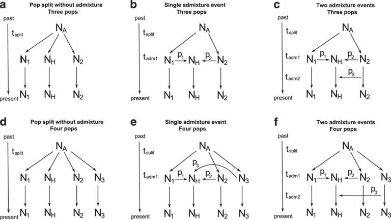
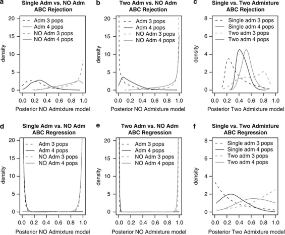
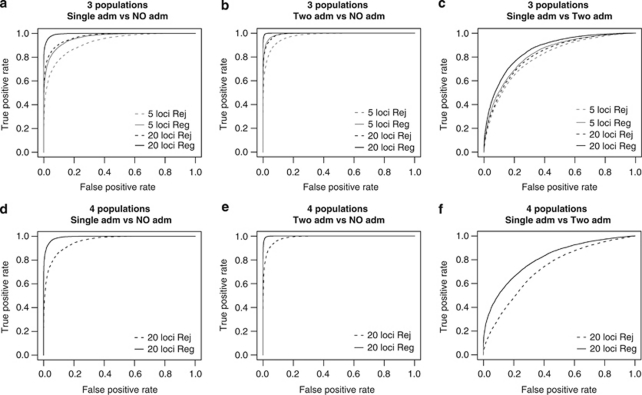
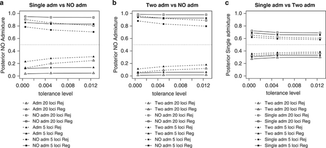
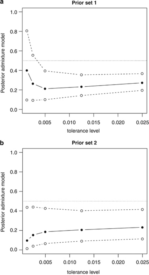
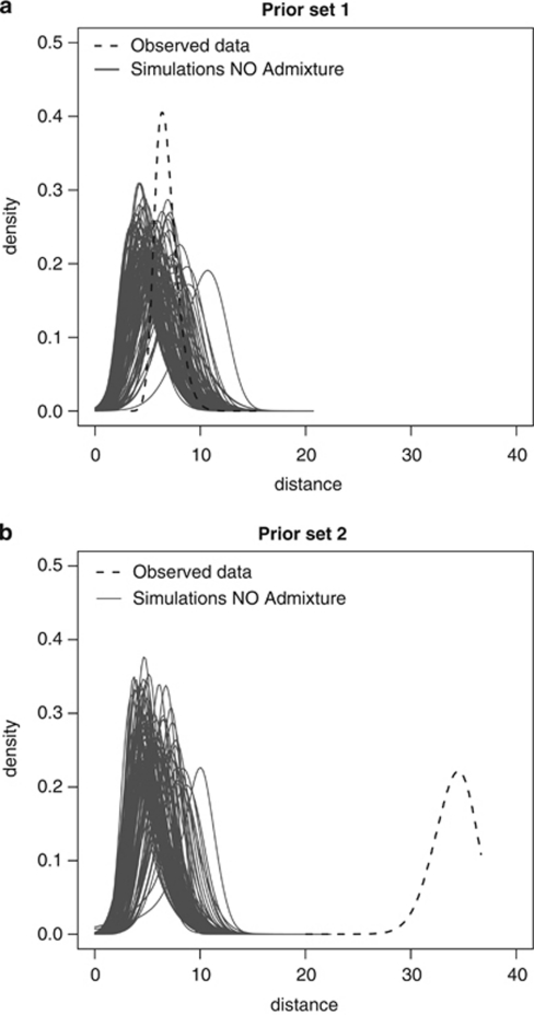
Genetic data have been widely used to reconstruct the demographic history of populations, including the estimation of migration rates, divergence times and relative admixture contribution from different populations. Recently, increasing interest has been given to the ability of genetic data to distinguish alternative models. One of the issues that has plagued this kind of inference is that ancestral shared polymorphism is often difficult to separate from admixture or gene flow. Here, we applied an approximate Bayesian computation (ABC) approach to select the model that best fits microsatellite data among alternative splitting and admixture models. We performed a simulation study and showed that with reasonably large data sets (20 loci) it is possible to identify with a high level of accuracy the model that generated the data. This suggests that it is possible to distinguish genetic patterns due to past admixture events from those due to shared polymorphism (population split without admixture). We then apply this approach to microsatellite data from an endangered and endemic Iberian freshwater fish species, in which a clustering analysis suggested that one of the populations could be admixed. In contrast, our results suggest that the observed genetic patterns are better explained by a population split model without admixture.


Figures

Figure 1
Figure 1
Admixture and population split models. (a) Population split model with three populations and without admixture. (b) Admixture model with two parental populations and one admixture event. (c) Admixture model with two parental populations and two admixture events. (d) Population split model with four populations and without admixture. (e) Admixture model with three parental populations and one admixture event. (f) Admixture model with three parental populations and two admixture events. In all models, the populations are allowed to have different effective sizes Ni, (i=1, 2, 3, H). The admixture and split events occurred at tadm1, tadm2 and tsplit generations ago.
Figure 2
Figure 2
Distribution of the posterior probabilities for the population split without admixture model (NO admixture; a, b, d, e), and for the two-event admixture model obtained with the simulated data sets (c, f). Each curve was obtained with the analysis of 10 000 simulated data sets. In (a), (b), (d) and (e), black lines correspond to data sets generated under the admixture models, whereas gray lines correspond to data sets generated under the NO admixture models. In (c) and (f), black lines correspond to data sets generated under the single-admixture models (single adm), and gray lines correspond to data sets generated under the two-event admixture models (two adm). Solid lines correspond to the four-population models and dashed lines to the three-population models. The simulated test data sets were simulated with parameters sampled from the priors of each model.
Figure 3
Figure 3
ROC analysis of the ABC method for the different scenarios tested. The top panel shows the ROC curves for the comparison of alternative models with three populations (ac), and the bottom panel for models with four populations (df). The curves compare the results obtained with a pure ABC rejection (dashed lines) and applying the logistic regression step (solid lines). For the three-population models, the curves obtained with 5 and 20 loci are shown as gray and black lines, respectively. (a) Single admixture versus no admixture (two parental); (b) two admixture events versus no admixture (two parental); (c) single admixture versus two admixture events (two parental); (d) single admixture versus no admixture (three parental); (e) two admixture versus no admixture (three parental); (f) single admixture versus two admixture (two parental).
Figure 4
Figure 4
Effect of tolerance and regression in the mean posterior distributions. (a, b) Average posterior distribution for the population split without admixture model (NO admixture) as a function of the tolerance, and average posterior distribution for the single-event admixture model (Single admixture) in (c). Each point represents the average of 10 000 posterior probabilities. The simulated test data sets were simulated with parameters sampled from the prior. The horizontal dotted line corresponds to the prior probability of 0.50, meaning that both models are equally likely.
Figure 5
Figure 5
Posterior probability for the single-event admixture model (admixture) obtained for I. lusitanicum, for the model comparison of single-event admixture vs population split without admixture. Posterior probabilities for the admixture model shown as function of the tolerance level, for: (a) results obtained with the first prior set; (b) results obtained with the second prior set. Solid lines correspond to the results obtained with the regression step and the dashed lines correspond to the 95% confidence interval. The horizontal dotted lines correspond to the prior probability of 0.50, meaning that both models are equally likely.
Figure 6
Figure 6
Comparison of the distance distributions between the I. lusitanicum data set and simulated data under the population split admixture model (NO admixture), with the distance distributions obtained for 100 data sets simulated under the most likely model (NO admixture). The simulated and observed data sets were compared with the same 10 000 simulations under the NO admixture model, with the parameters values sampled from the prior distributions. This model was selected as the most likely given the I. lusitanicum data. (a) Analysis with the first prior set tested; (b) analysis with the second prior set tested (see text for details).

Similar articles

Cited by

References

    1. Alves MJ, Coelho MM. Genetic variation and population subdivision of the endangered Iberian cyprinid Chondrostoma lusitanicum. J Fish Biol. 1994;44:627–636.
    1. Bazin E, Dawson KJ, Beaumont MA. Likelihood-free inference of population structure and local adaptation in a Bayesian hierarchical model. Genetics. 2010;185:587–602. - PMC - PubMed
    1. Beaumont M. Approximate Bayesian computation in evolution and ecology. Annu Rev Ecol Evol Syst. 2010;41:379–406.
    1. Beaumont MA.2008. Joint determination of tree topology and population history. In: Matsumura S, Forster P, Renfrew C (eds) Simulation, Genetics, and Human Prehistory. McDonald Institute for Archaeological Research: Cambridge; 135–154.
    1. Beaumont MA, Nielsen R, Robert C, Hey J, Gaggiotti O, Knowles L, et al. In defence of model-based inference in phylogeography. Mol Ecol. 2010;19:436–446. - PMC - PubMed

Publication types