. 2011;6(12):e28766.
doi: 10.1371/journal.pone.0028766. Epub 2011 Dec 7.

Protein 3D structure computed from evolutionary sequence variation

Affiliations

Protein 3D structure computed from evolutionary sequence variation

Debora S Marks et al. PLoS One. 2011.

Abstract

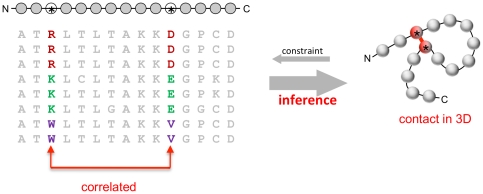
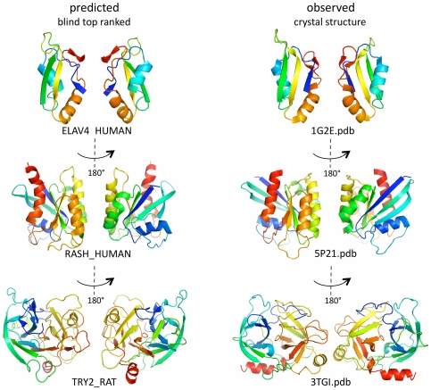
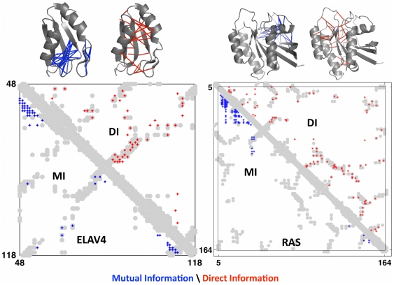
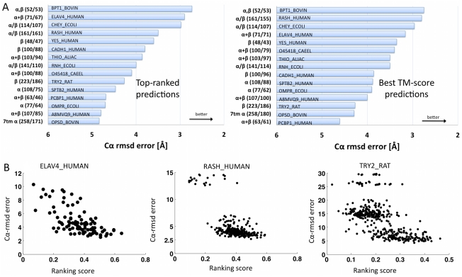
The evolutionary trajectory of a protein through sequence space is constrained by its function. Collections of sequence homologs record the outcomes of millions of evolutionary experiments in which the protein evolves according to these constraints. Deciphering the evolutionary record held in these sequences and exploiting it for predictive and engineering purposes presents a formidable challenge. The potential benefit of solving this challenge is amplified by the advent of inexpensive high-throughput genomic sequencing.In this paper we ask whether we can infer evolutionary constraints from a set of sequence homologs of a protein. The challenge is to distinguish true co-evolution couplings from the noisy set of observed correlations. We address this challenge using a maximum entropy model of the protein sequence, constrained by the statistics of the multiple sequence alignment, to infer residue pair couplings. Surprisingly, we find that the strength of these inferred couplings is an excellent predictor of residue-residue proximity in folded structures. Indeed, the top-scoring residue couplings are sufficiently accurate and well-distributed to define the 3D protein fold with remarkable accuracy.We quantify this observation by computing, from sequence alone, all-atom 3D structures of fifteen test proteins from different fold classes, ranging in size from 50 to 260 residues, including a G-protein coupled receptor. These blinded inferences are de novo, i.e., they do not use homology modeling or sequence-similar fragments from known structures. The co-evolution signals provide sufficient information to determine accurate 3D protein structure to 2.7-4.8 Å C(α)-RMSD error relative to the observed structure, over at least two-thirds of the protein (method called EVfold, details at http://EVfold.org). This discovery provides insight into essential interactions constraining protein evolution and will facilitate a comprehensive survey of the universe of protein structures, new strategies in protein and drug design, and the identification of functional genetic variants in normal and disease genomes.


Conflict of interest statement

Competing Interests: The authors have declared that no competing interests exist.

Figures

Figure 1
Figure 1. Correlated mutations carry information about distance relationships in protein structure.
The sequence of the protein for which the 3D structure is to be predicted (each circle is an amino acid residue, typical sequence length is 50–250 residues) is part of an evolutionarily related family of sequences (amino acid residue types in standard one-letter code) that are presumed to have essentially the same fold (iso-structural family). Evolutionary variation in the sequences is constrained by a number of requirements, including the maintenance of favorable interactions in direct residue-residue contacts (red line, right). The inverse problem of protein fold prediction from sequence addressed here exploits pair correlations in the multiple sequence alignment (left) to deduce which residue pairs are likely to be close to each other in the three-dimensional structure (right). A subset of the predicted residue contact pairs is subsequently used to fold up any protein in the family into an approximate predicted 3D shape (‘fold’) which is then refined using standard molecular physics techniques, yielding a predicted all-atom 3D structure of the protein of interest.
Figure 2
Figure 2. Predicted 3D structures for three representative proteins.
Visual comparison of 3 of the 15 test proteins (others in Figure S3) reveals the remarkable agreement of the predicted top ranked 3D structure (left) and the experimentally observed structure (right). Center: Cα-RMSD error and, in parentheses, number of residues used for Cα-RMSD error calculation, e.g., 2.9 Å Cα-RMSD (67). The ribbon representation was chosen to highlight the overall topographical progression of the polypeptide chain, rather than atomic details such as hydrogen bonding (colored blue to red in rainbow colors along the chain, N-term to C-term; helical ribbons are α-helices, straight ribbons are β-strands, arrow in the direction of the chain; each structure in front and back view, related by 180 degree rotation). The predicted proteins can be viewed in full atomic detail in deposited graphics sessions for the Pymol program (Web Appendix A4) or from their coordinates (Web Appendix A).
Figure 3
Figure 3. Progress in contact prediction using the maximum entropy method.
Extraction of evolutionary information about residue coupling and predicted contacts from multiple sequence alignments works much better using the global statistical model (right, Direct Information, DI, Equation 3) than the local statistical model (left, Mutual Information, MI, Equation 1). Predicted contacts for DI (red lines connecting the residues predicted to be coupled from sequence information) are better positioned in the experimentally observed structure (grey ribbon diagram), than those for MI (left, blue lines), shown here for the RAS protein (upper) and ELAV4 protein (lower). The DI residue pairs are also more evenly distributed along the chain and overlap more accurately with the contacts in the observed structure (red stars [predicted, grey circles [observed] in contact map; center, upper right triangle) than those using MI (blue [predicted], grey circles [observed]; center, lower left triangle). Details of contact maps for all proteins comparing predicted and observed contacts are in Figures S1 and S2, Text S1.
Figure 4
Figure 4. Accuracy of blinded 3D structure inference.
A. The overall performance of the de novo structure prediction reported here based on contacts inferred from evolutionary information (EICs), ranges from good to excellent for the 15 test proteins (on left: 3D structure type [α = α-helix-containing, β = β-strand-containing, 7tm-α = containing seven trans-membrane helices]; in parentheses: size of protein domain/number of residues used for Cα-RMSD error calculation; on bar: Uniprot database ID). Larger bars mean better performance, i.e., lower Cα-RMSD co-ordinate error. Left: performance for the top ranked structure for each target protein out of 400–560 (depending on the size of the protein, 20 structures per NC bin, NC in steps of 10, details in Appendix A3 and A6) candidate structures in blind prediction mode; right: performance of the best structure, in hindsight, out of 20 candidate structures generated, for 20 sets of constraints ranging from 10∶200, in steps of 10. This reflects what would be achievable with better ranking criteria or independent post-prediction validation of structure quality (Table 1; details of blind ranking scores in Web Appendix A5). Other well-accepted methods for error assessment, such as GDT-TS and TM score are useful for comparison purposes (Table S1, Web Appendix A6). B. Ranking score of each candidate structure (quantifying expected structure quality) versus Cα-RMSD error. Ideally, higher-ranking scores correspond to lower error. The distribution of the candidate structures (black dots) for Elav4, Ras and Trypsin shows, in retrospect, that the ranking criteria used here are relatively useful and help in anticipating which structures are likely to be best (plots for all tested proteins in Figure S5). In blind prediction mode, a list of predicted candidate 3D structure has to be ranked by objective and automated criteria, with a single top ranked structure or a set of top ranked structures nominated as preferred predictions.
Figure 5
Figure 5. Top-ranked predicted structures can make correct contacts in the absence of constraints and avoid incorrect contacts in spite of false positive constraints.
The top blindly ranked structures are evaluated in terms of quality of contact prediction (NC = 40 for Elav4, NC = 130 for Ras, NC = 160 for Trypsin). The predicted constraints (red stars) are correct when they coincide with contacts derived from the observed structure (grey circles) and otherwise incorrect (false positives, red on white). The contacts derived from the predicted 3D structure (dark blue) are in good general agreement with those from the observed structure (grey). The cooperative nature of the folding prediction process permits favorable situations, in which contacts regions not touched by a predicted constraint (red) are still predicted correctly (black circle for RAS, dark blue on grey, no red) and false positive constraints are not strong enough to lead to incorrect contacts (left black circle Elav4, red star, no dark blue or grey). However, in unfavorable situations missing constraints may imply that contact regions are fully or partially missed (black circle, trypsin) or mostly missed (right black circle for Elav4, grey adjacent to and wider than dark blue).
Figure 6
Figure 6. Key requirement of global statistical model for correct prediction.
Evaluation of accuracy in terms of predicted contacts (A) and predicted 3D structures (B). (A) The two global models, the Bayesian network model (BNM, green [13]) and direct information model (DI, red, this work and [47]) have a consistently high rate of correctly predicted contacts (true positives) among the top NC ranked residue pairs; two local models, mutual information (MI, green, equation 1) and SCA (black, [66]) have a consistently lower rate of true positives. Here, local refers to statistical independence of each pair i,j, while global refers to statistical consistency of all pairs. In (B), only the predicted 3D structures (green, BNM; red, EIC) for the global models agree well with the observed structure (grey); Cα-RMSDs is calculated over the number or residues in parentheses (Pymol sessions for all structures in Web Appendix A4). Attempts to generate 3D structures for the two local methods MI and SCA failed (not shown). Comparing (A) and (B) confirms that a higher rate of true positives for contact prediction leads to better 3D structures and that for DI one needs at least a true positive rate of about 0.5 for about 100 predicted contacts, depending on size and other details of particular protein families. Interestingly, a false positive rate as high as about 0.3–0.5 can still be consistent with good 3D structure prediction.
Figure 7
Figure 7. Moderate number of distance constraints and varying number of sequences required for correct 3D structure prediction.
A. How many distance constraints are needed for fold prediction? What fraction of false positives can be tolerated? With increasing number of predicted essential distance constraints (NC, horizontal axis), 3D prediction error decreases rapidly, as assessed by Cα-RMSD between the best of 20 (in each NC bin) predicted structures and the observed structure (here, for the 15 test proteins, using Pymol). Remarkably, as few as ∼NRES/2 (∼L/2) distance constraints dij (with chain distance |i−j|>5) suffice for good quality predictions below 5 Å Cα-RMSD, where NRES is the number of amino acid residues in the protein multiple sequence alignment. We therefore routinely generated candidate protein structures for up to NC = NRES distance constraints for blinded ranking (and for up to NC = 200 for other tests). Eventually the number of false positives does degrade prediction quality, e.g., for the 58 residue protein BPTI once NC is about 80 (1.5 NRES) the prediction quality is lost. In practice, we do not recommend using NC>NRES, i.e, more than about one constraint dij with |i−j|>5, per residue. B. When would it have been possible to fold from sequence? The increase in the number of sequences available in public databases (here, from successive archival releases of the PFAM collection of protein family alignments) is one of two key elements in the ability to predict protein folds from correlated mutations. Nevertheless plotting the numbers of sequences and dates shows that it would have been possible to calculate the structures up to 10 years ago for some proteins and that amazingly few sequences are sufficient. For example, although the retrospective prediction error (vertical axis, Cα-RMSD, using Pymol) for the best 3D structure (of 400 candidates each) in four protein families (Ras, SH3 domain (YES_human) and RnaseH from Ecoli) has decreased over time, the decrease is not strictly monotonic, as the result of non-systematic growth of the database. The point at which a predicted protein structure from a particular family reaches below 4 Å Cα-RMSD varies considerably. For example, while RnaseH required about 6000 sequence to dip below 4 Å error, reached around 2008, the structure of CheY could have been predicted to 3.3 Å Cα-RMSD, with only the 600 sequences available in 1999.
Figure 8
Figure 8. Computational pipeline for protein folding.
The MSA for the protein family is typically generated by a sequence similarity search in a large database of protein sequences to collect related sequences that are likely to have similar 3D structures. Correlations between sequence positions i and j are calculated from observed frequencies of amino acids in single MSA columns and column pairs. By inferring a minimal statistical model of full length-sequences, which is consistent with these correlations (Text S1), direct coupling strengths eij(A,B) between any pairs of residues are deduced. They help to derive distance constraints, which in turn are used to produce folded structures using the following steps: distance geometry generation of approximate folds, molecular dynamics simulated annealing using standard force fields, and chirality filtering. Here, we use MSAs from the PFAM collection of pre-aligned sequence families .

References

    1. Finn RD, Mistry J, Tate J, Coggill P, Heger A, et al. The Pfam protein families database. Nucleic Acids Res. 2010;38:D211–222. - PMC - PubMed
    1. Altschuh D, Lesk AM, Bloomer AC, Klug A. Correlation of co-ordinated amino acid substitutions with function in viruses related to tobacco mosaic virus. J Mol Biol. 1987;193:693–707. - PubMed
    1. Miller CS, Eisenberg D. Using inferred residue contacts to distinguish between correct and incorrect protein models. Bioinformatics. 2008;24:1575–1582. - PMC - PubMed
    1. Altschuh D, Vernet T, Berti P, Moras D, Nagai K. Coordinated amino acid changes in homologous protein families. Protein Eng. 1988;2:193–199. - PubMed
    1. Göbel U, Sander C, Schneider R, Valencia A. Correlated mutations and residue contacts in proteins. Proteins. 1994;18:309–317. - PubMed

Publication types