The role of exploratory conditions in bio-inspired tactile sensing of single topogical features

Abstract

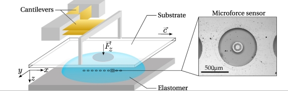
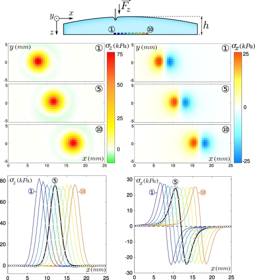
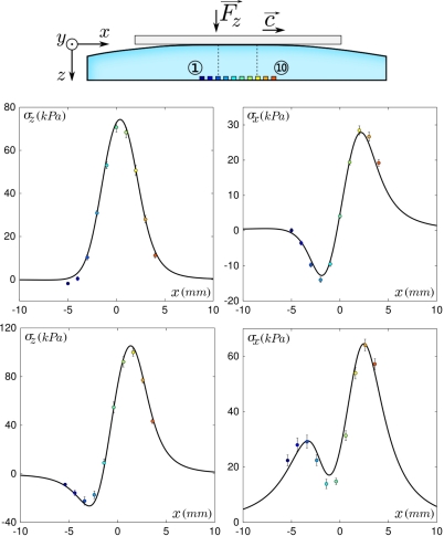
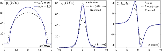
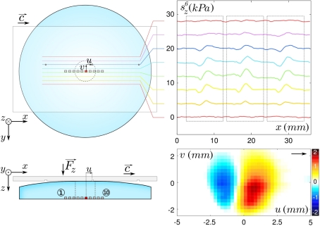
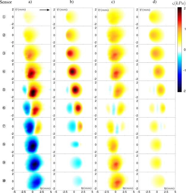
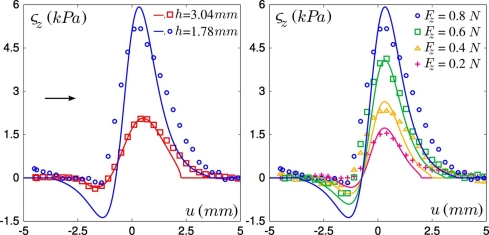
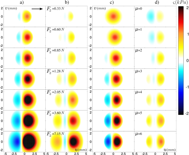
We investigate the mechanism of tactile transduction during active exploration of finely textured surfaces using a tactile sensor mimicking the human fingertip. We focus in particular on the role of exploratory conditions in shaping the subcutaneous mechanical signals. The sensor has been designed by integrating a linear array of MEMS micro-force sensors in an elastomer layer. We measure the response of the sensors to the passage of elementary topographical features at constant velocity and normal load, such as a small hole on a flat substrate. Each sensor's response is found to strongly depend on its relative location with respect to the substrate/skin contact zone, a result which can be quantitatively understood within the scope of a linear model of tactile transduction. The modification of the response induced by varying other parameters, such as the thickness of the elastic layer and the confining load, are also correctly captured by this model. We further demonstrate that the knowledge of these characteristic responses allows one to dynamically evaluate the position of a small hole within the contact zone, based on the micro-force sensors signals, with a spatial resolution an order of magnitude better than the intrinsic resolution of individual sensors. Consequences of these observations on robotic tactile sensing are briefly discussed.

Keywords: MEMS tactile sensor array; biomimetic sensor; friction; human tactile perception; hyperacuity; mechanoreceptors; receptive field; topological feature localization.

Figure 1.

Scheme of the tactile sensing device and blow-up image of one individual micro-force sensor. (Left) Sketch of the experimental setup. The sensing device is made of a linear array of 10 MEMS micro-force sensors mounted on a rigid base (lower gray block), covered with a PDMS spherical cap. Flat substrates or indentor (in the form of a small rod, not shown) can be displaced and applied onto the surface of the sensing device. (Right) Picture of one MEMS micro-force sensor as seen from above.

Figure 2.

Characterization of the intrinsic receptive fields. (Top) Sketch showing the local indentation procedure. A 500 μm in diameter cylinder is indented at the surface of the elastomer cap at varying positions (x, y). (Middle) Normal (left) and tangential (right) stress fields, respectively σ_z and σ_x, measured by the micro-force sensors ①, ⑤ and ⑩ as a function of the indentor’s position (x, y) under a unit normal force F_z =1 N. (Bottom) Normal (left) and tangential (right) stress measured by each of the 10 micro-force sensors (from blue to red) as a function of the indentor’s position x for y =0 under a unit normal force and for a layer thickness h =3.04 mm. The experimental stress measured by sensor ⑤ (white circles) is compared to the prediction of a Finite Element calculation (black solid curve).

Figure 3.

Static and dynamical mean stress as measured by the sensors and compared to the model’s predictions for a flat substrate. (Top) Sketch: a flat substrate is rubbed against the surface of the sensing device with a normal force F_z =0.8 N(h =3.04 mm). Vertical dashed lines represent the boundaries of the contact zone and scale with the actual sensors’ locations. (Middle) Averaged stress versus sensors location x in the static regime (c =0) for the 10 sensors (colored circles) compared to the model’s prediction (black curve) for the normal component σ_z (left) and similarly for the tangential component σ_x along the direction of motion (right). Position x =0 is the center of the contact. Error bars show the measured standard deviation and colors correspond to the locations depicted on the upper sketch. (Bottom) Same as above but in the steady sliding regime (c = 500 μ m/s).

Figure 4.

Effect of the finite thickness of the elastic layer. (Left) Sphere-on-plane contact pressure profile calculated for a semi-infinite elastic medium (Hertz’ calculation, dashed black line) and an elastic layer of thickness h (blue line) such that h/a =1.3 where a is the contact radius. This ratio corresponds to the experimental conditions. (Center-Right) Normal component g_zz (center) and tangential component g_xz (right) of the Green tensor in (x, y =0, z = h): the profile for the semi-infinite layer (dashed line) can be rescaled (blue line) to approximate the profile obtained by Finite Elements simulation for a layer of thickness h =3.04 mm (dotted line).

Figure 5.

Generation of the Exploratory Receptive Fields (ERF). (Left) Sketches of the scanning protocol for lines of isolated defects (top: top view, bottom: side view). Dashed circle and lines represent the boundaries of the contact zone, which scale with the actual sensors’ locations. The substrate moves at constant velocity c. The relative position of the nearest defect to a given sensor is denoted (u(t), v(t)). Right-Top Normal stress responses to 3 successive defects for sensor ⑥ (h =3.04 mm, F_z =0.8 N, c = 500 μ m/s). The raw signals, converted in stress unit, are shown for only 8 scanning lines and are shifted vertically from one to the next for clarity. Right-Bottom ERF of the normal stress ς_z for sensor ⑥, reconstructed from the average of 14 responses to defects. Color code units are kPa.

Figure 6.

Measured and predicted ERF. Each row corresponds to one sensor, from ① to ⑩ starting from the top. Each column corresponds to the measured (a) and predicted (b) normal stress ς_z, and measured (c) and predicted (d) shear stress ς_x. Standard deviations are typically 0.6 kPa for σ_z and 0.4 kP a for σ_x. The arrow indicates the defect’s displacement. The color code is the same for all plots. h =3.04 mm and F_z =0.8 N.

Figure 7.

Role of two exploratory parameters: experimental data (points) at the ERF median line (v =0) are compared to the model prediction (solid curves) for a sensor at the center of the contact. (Left) Average normal stress variations σ_z for two layer thicknesses: h =1.78 mm (blue circles) and h =3.04 mm (red squares). The arrow indicates the defect’s displacement. F_z =0.8 N. (Right) Average normal stress variations σ_z for four normal forces from 0.2 to 0.8 N (h =1.78 mm).

Figure 8.

Evolution of the predicted ERF for a sensor at the center of the contact zone (x =0, y =0) in response to a single defect in (u, v) scanned at constant speed from left to right (h =3.04 mm, c = 500 μ m/s). Two parameters are explored: (a–b) the applied normal force F_z and (c–d) the dynamic friction coefficient μ_d. Columns (a) and (c) show the normal stress profiles σ_z, columns (b) and (d) show the shear stress profiles in the direction of motion σ_x.

Figure 9.

Detection of the defect’s position along the direction of motion. (Left) Distance between the actual and predicted positions of the defect δu_z for 500 random positions of the defect in the contact zone. The predicted positions are derived by comparing the measured normal stress signals to the average stress profiles for 1, 2 and 5 sensors chosen at random for each realization. The dashed horizontal lines on all three plots are boundaries of the contact zone. (Right) Prediction accuracy s^u as a function of the number of sensors used when only the shear stress signal is used ( $s_x^u$, green circles), then when only the normal stress is used ( $s_z^u$, blue squares) and finally when both signals are used ( $s_{\mathit{xz}}^u$, black triangles). In all three cases, the prediction accuracy converges asymptotically to 150 μm.

References

1. Hollins M. Somesthetic senses. Annu. Rev. Psychol. 2010;61:243–271. - PubMed
1. Johansson R, Flanagan J. Coding and use of tactile signals from the fingertips in object manipulation tasks. Nat. Rev. Neurosci. 2009;10:345–59. - PubMed
1. Westling G, Johannson RS. Factors influencing the force control during precision grip. Exp. Brain Res. 1984;53:277–284. - PubMed
1. Dahiya RS, Metta G, Valle M, Sandini G. Tactile sensing—From humans to humanoids. IEEE Trans. Rob. 2010;26:1–20.
1. Maheshwari V, Saraf RF. High-resolution thin-film device to sense texture by touch. Science. 2006;312:1501–1504. - PubMed
Publication types
LinkOut - more resources