. 2011 Dec 14;31(50):18506-21.
doi: 10.1523/JNEUROSCI.2974-11.2011.

Local diversity and fine-scale organization of receptive fields in mouse visual cortex

Affiliations

Local diversity and fine-scale organization of receptive fields in mouse visual cortex

Vincent Bonin et al. J Neurosci. .

Abstract

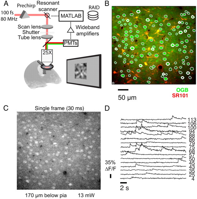
Many thousands of cortical neurons are activated by any single sensory stimulus, but the organization of these populations is poorly understood. For example, are neurons in mouse visual cortex--whose preferred orientations are arranged randomly--organized with respect to other response properties? Using high-speed in vivo two-photon calcium imaging, we characterized the receptive fields of up to 100 excitatory and inhibitory neurons in a 200 μm imaged plane. Inhibitory neurons had nonlinearly summating, complex-like receptive fields and were weakly tuned for orientation. Excitatory neurons had linear, simple receptive fields that can be studied with noise stimuli and system identification methods. We developed a wavelet stimulus that evoked rich population responses and yielded the detailed spatial receptive fields of most excitatory neurons in a plane. Receptive fields and visual responses were locally highly diverse, with nearby neurons having largely dissimilar receptive fields and response time courses. Receptive-field diversity was consistent with a nearly random sampling of orientation, spatial phase, and retinotopic position. Retinotopic positions varied locally on average by approximately half the receptive-field size. Nonetheless, the retinotopic progression across the cortex could be demonstrated at the scale of 100 μm, with a magnification of ≈ 10 μm/°. Receptive-field and response similarity were in register, decreasing by 50% over a distance of 200 μm. Together, the results indicate considerable randomness in local populations of mouse visual cortical neurons, with retinotopy as the principal source of organization at the scale of hundreds of micrometers.


Figures

Figure 1.
Figure 1.
Wide-field, video-rate, two-photon imaging in mouse visual cortex. A, In vivo imaging preparation. Mice were anesthetized and their heads held fixed while visual stimuli were displayed to the contralateral eye. For imaging, short infrared laser pulses (100 fs) were raster scanned (frame rate 31 Hz) onto the brain using a resonant galvanometric system (8000 lines/s, 240 lines per frame) through a high-NA water-immersion objective lens. Emitted light was collected with GaAsP photomultipliers (PMTs) and acquired using a multifunction board (0.3 μs/sample). Images were reconstructed on-line in MATLAB and streamed onto a disk array (RAID). B, Typical imaged plane showing neurons (green) and astrocytes (yellow) labeled with calcium indicator OGB-1 and sulforhodamine 101 (SR101). Overlaid contours (gray and white) indicate manually segmented neuron cell bodies. C, Single-image frame (green channel) showing that cell bodies and blood vessels are visible at 30 ms time scale (170 μm below pia, 13 mW average power). D, Somatic calcium time courses obtained by summing pixels over cell bodies, for 16 of the 114 labeled neurons (B, thick contours). At these low laser powers, a slow decay of fluorescence and transient amplitude was observed (see Results).
Figure 2.
Figure 2.
Estimating spike-related calcium activity in the face of motion and neuropil contamination. A, Frame-to-frame x-y brain displacement in polar coordinates estimated from rigid registration of the image stack to the average frame. B1, Correction for motion in depth (z-motion) and neuropil contamination. Somatic fluorescence time courses of two nearby cells obtained from registered stack (first row), estimated z-motion component (second row), estimated neuropil component (third row), and corrected time courses (fourth row, black). Note how the correction captures the effect of z-motion on the cells' time courses. Model somatic calcium fluorescence (fourth row, red curves) and firing events (fourth row, red ticks, ΔF/F > 3.0%, 30 ms bins) inferred using a fast non-negative deconvolution algorithm (Vogelstein et al., 2010). B2, Validation of the method of Vogelstein et al. (2010) on simultaneous calcium imaging and cell-attached recordings in mouse visual cortex in vivo. Raster plots (500 ms bins) show calcium transient rates (top) and measured firing (bottom) rates of a regular-spiking (putative excitatory) neuron. Data from a previous study (Kerlin et al., 2010). C, Uncorrected versus corrected time courses. Half the imaged cells are shown for clarity. The correction removes the common, periodic signals that contaminate the raw somatic time courses. D, Amplitude spectra of uncorrected time courses (top, black), estimated z-motion components (D1, red), and estimated neuropil components (D1, blue). In the z-motion component, effects of breathing (<2 Hz) and heart beat (9 Hz) are visible. In the neuropil component, rhythmic calcium activity (<2 Hz) and ambient light (7 Hz). The corrected time courses (D2, thick line) have an exponential spectrum, which was well described by the deconvolution method (D2, red), as inferred by the flat spectrum of the residuals [corrected—model] (D2, gray). E, Pairwise correlation between estimated firing of simultaneously imaged neurons before (E1) and after correction (E2). Stem plot (E3) compares a single row of the correlation matrices (E1, E2, arrow). Correcting for motion and neuropil reveals the sparse correlation structure of responses. C, E, Data from Figure 1. A, B, D, Data from Figures 4–8.
Figure 3.
Figure 3.
Spatial summation in excitatory and inhibitory neurons. Experiments in visual cortex of GAD67-GFP knock-in mice in which all GABAergic inhibitory interneurons are labeled with green fluorescent protein (Tamamaki et al., 2003). Stimuli were sinusoidal gratings moving at 1 Hz in 8–12 different directions interleaved with periods of isoluminant gray screen. A, Trial average somatic calcium responses (black traces) and transient rates (red histograms) for five excitatory (A1) and five inhibitory neurons (A2) (averaged across five repetitions). Vertical lines indicate stimulus onset and offset. Excitatory neurons were highly selective for a narrow range of stimulus orientations and often showed pronounced periodic responses to these stimuli. GABAergic interneurons were nonselective or weakly selective and exhibited little periodicity in their responses. B, Single-trial responses of an excitatory neuron (closed circle) and an inhibitory interneuron (open circle, same data as in A, dashed boxes). C, For the same neurons, tonic (open symbols) and periodic (close symbols) components of responses as a function of stimulus direction. Error bars indicate SE. D, Modulation versus tuning indices for 262 neurons (N = 4 planes from two animals). Data points for each imaged plane depicted with different symbols. Excitatory neurons (red) and interneurons (blue) show distinct functional properties.
Figure 4.
Figure 4.
Characterizing excitatory neurons with wavelet stimuli. A, Wavelet stimulus made of random, localized, oriented stimuli of different positions, sizes, and directions. The stimulus is generated by applying the inverse 3D wavelet transform to sparse random coefficients. B, Single-trial calcium time courses (black) and inferred firing activity (red) for 7 of 82 imaged cells (one imaged plane). Stimulus consists of ∼16 s epochs of wavelets preceded by ∼8 s periods of gray screen (16 different stimuli for a total of ∼400 s per trial). Same experiment as in Figure 2, A, B1, and D, and Figures 5–8. C, Same experiment, average fraction of neurons active (top) and fraction of trials active as function of time (bottom) (ΔF/F > 3.0%, 500 ms bins). D, Triggered averages computed by calculating the cross-correlation between the stimulus and the response (ΔF/F > 3.0%), and by comparing results between stimulus repetitions. E, Receptive fields often have elongated ON (red) and OFF (blue) subregions characteristic of simple cells. F, Receptive fields estimated from successive sets of trials are similar (20 min of imaging each; cell 14). G, Comparison to responses to moving grating stimuli. Orientation tuning (black lines) and preference (red lines) inferred from receptive-field mapping is consistent with that measured with drifting gratings.
Figure 5.
Figure 5.
Receptive-field modeling. A, Model of responses consisting of a linear filter (a Gabor filter in space and a gamma function in time) and a rectifying nonlinearity. B, Fitted linear filter for neuron in Figure 4D (cell 14, note change in color scale in Fig. 4D). C, Measured (black line) and model responses (red line). For this cell, the model fit explains ∼12% of the stimulus-evoked variance in the responses. Responses were smoothed with a Gaussian filter (σ = 30 ms). D, Example estimated spatial receptive fields. Event-triggered averages (top rows, as computed in Fig. 4) and estimated spatial linear filters (bottom rows). Only fits that explain >10% of the stimulus-evoked variance are shown. From these fits, we can extract parameters such as receptive-field position, size, and orientation.
Figure 6.
Figure 6.
Local diversity and organization of spatial receptive fields. A, Model spatial receptive fields (RFs) overlaid on a schematic view of cortex (gray contours) to illustrate relationship between RF position and neuron location in cortex. Lines point to the cell bodies of neurons from which the RFs were recorded. Only a subset of the most significant RFs are shown (absolute mean/SE >5.0% and explained variance >5%, n = 50/82 cells). Receptive fields with different properties are intermingled. Note the shift in receptive-field position with neuron location (left to right, see Fig. 7). B, Average RF in imaged plane. ON and OFF RF subregions were biased toward distinct regions of visual space, but segregation was not strict, as evidenced by the diversity seen in A and by the small magnitude of the average (peak ∼0.25). C, Receptive-field similarity versus distance between cell bodies. Similarity defined as the normalized dot product between RFs. D, Cumulative distributions of pairwise RF similarity for neurons <100μm part (black), for neurons 100–250 μm apart (gray), and for all neurons combined (dashed). E, Cumulative distributions of RF similarity for measured (black) and surrogate RFs (gray). Surrogate RFs obtained by assigning random orientations or phases to the measured RFs. Results for multiple randomized sets are overlaid. Only significant RFs are considered.
Figure 7.
Figure 7.
Local retinotopic organization. A, Field of view with characterized neurons (circles). Only fits that explain >5% of the stimulus-evoked variance are considered (N = 50/82 neurons). B, Cell body positions (circles) and receptive-field centers relative to stimulus center (color-coded) along azimuth (left) and elevation (right). Vectors ν1 and ν2 denote the perpendicular axes along which RF azimuth and elevation show the largest shifts. C, Receptive-field positions (left), estimated retinotopic map (middle), and positional scatter (right). Maps show cell body (circles) and receptive-field centers (arrows; see inset on right). Retinotopic map defined as the rigid transformation of cortical space that minimized total square error of positions. D, Projection of retinotopic map (lines) and positions (circles) along vectors ν1 (left) and ν2 (right). For this dataset, cortical magnification is 5.1 μm/° along ν1 and 10.1 μm/° along ν2. E, Receptive-field overlap versus distance between cell bodies. Overlap defined as the ratio of shared receptive-field area over the area of the smaller receptive field. Area calculated from the width of the Gaussian envelope (full-width at half-maximum). Error bars indicate SE.
Figure 8.
Figure 8.
Receptive fields and activity correlations. A, Signal trial calcium responses (black) of two excitatory neurons with similar spatial receptive fields (insets) and inferred firing (red, >3% ΔF/F) for three repetitions of the wavelet stimulus. B, Distribution of signal correlations. Signal correlation defined as correlation coefficient between trial-average responses of pairs of neurons at zero lag minus the correlation lagged by 1 bin (500 ms bins). The calculated signal correlation for the cell pair shown in A is 0.35 ± 0.08 (mean ± SD bootstrap). C–F, Average signal correlation (black lines and symbols) versus absolute distance in receptive-field position (C), absolute difference in receptive-field orientation (D), receptive-field similarity (E), and distance between cell bodies (F). Gray dots in E show individual neuron pairs. Error bars indicate SE. G, Histogram shows average signal correlation as function of cortical distance and receptive-field similarity. For a given degree of similarity, correlation is approximately constant.

References

    1. Alonso JM, Usrey WM, Reid RC. Rules of connectivity between geniculate cells and simple cells in cat primary visual cortex. J Neurosci. 2001;21:4002–4015. - PMC - PubMed
    1. Andermann ML, Kerlin AM, Reid RC. Chronic cellular imaging of mouse visual cortex during operant behavior and passive viewing. Front Cell Neurosci. 2010;4:3. - PMC - PubMed
    1. Bandyopadhyay S, Shamma SA, Kanold PO. Dichotomy of functional organization in the mouse auditory cortex. Nat Neurosci. 2010;13:361–368. - PMC - PubMed
    1. Barlow HB. Possible principles underlying the transformation of sensory images. In: Rosenblith WA, editor. Sensory communication. Cambirdge, MA: MIT; 1961.
    1. Bock DD, Lee WC, Kerlin AM, Andermann ML, Hood G, Wetzel AW, Yurgenson S, Soucy ER, Kim HS, Reid RC. Network anatomy and in vivo physiology of visual cortical neurons. Nature. 2011;471:177–182. - PMC - PubMed

Publication types

LinkOut - more resources