Modeling the impact of common noise inputs on the network activity of retinal ganglion cells

Abstract

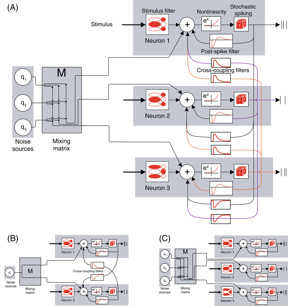
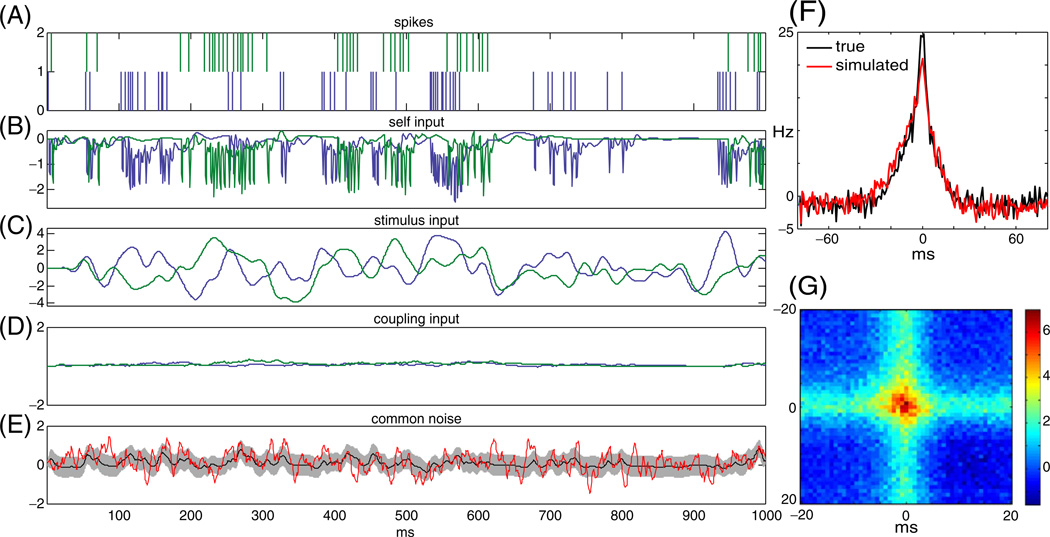
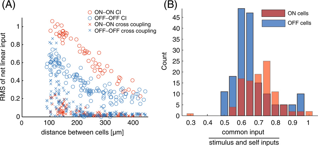
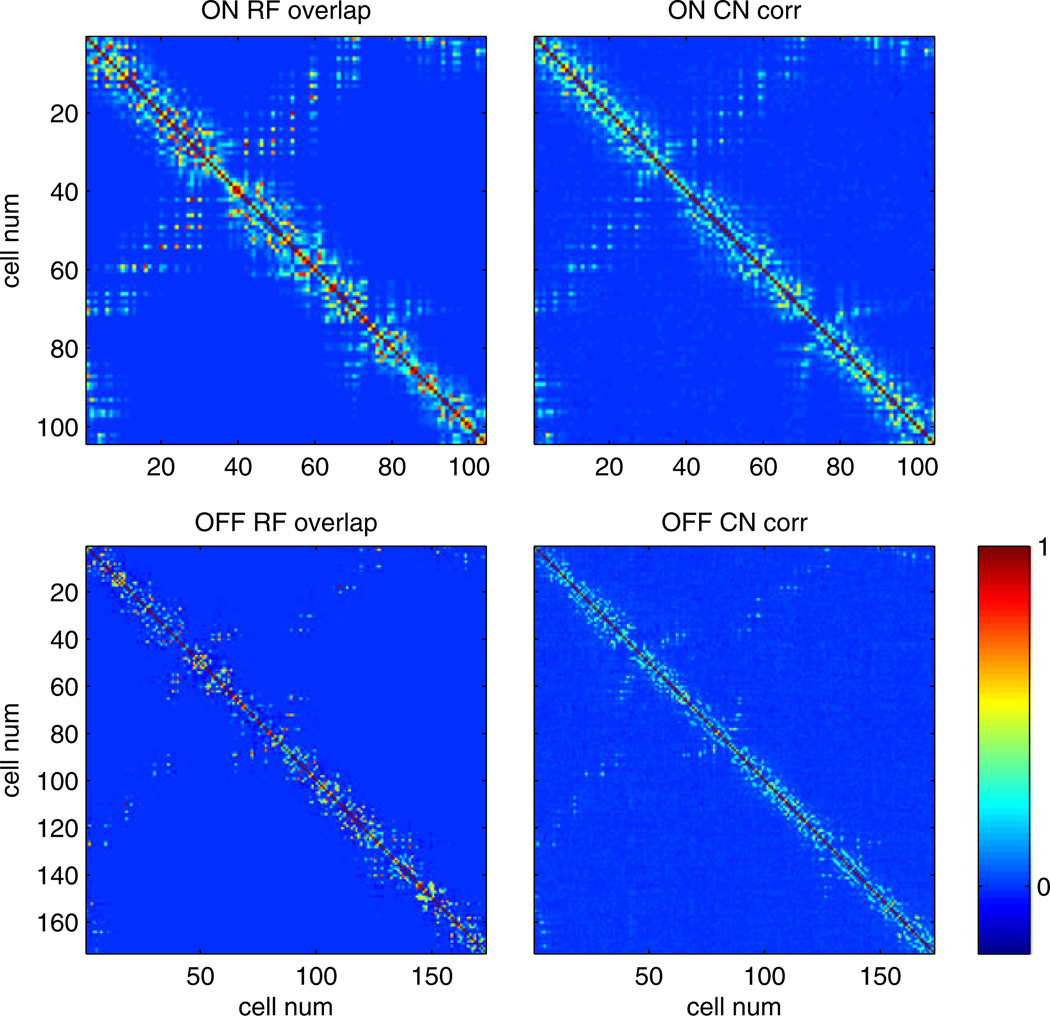
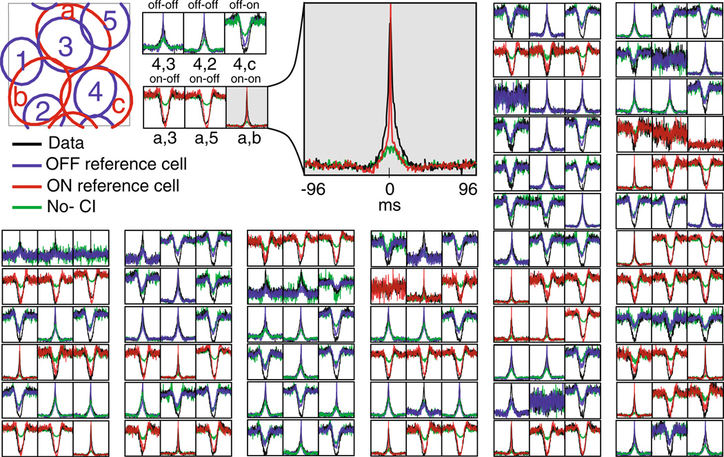
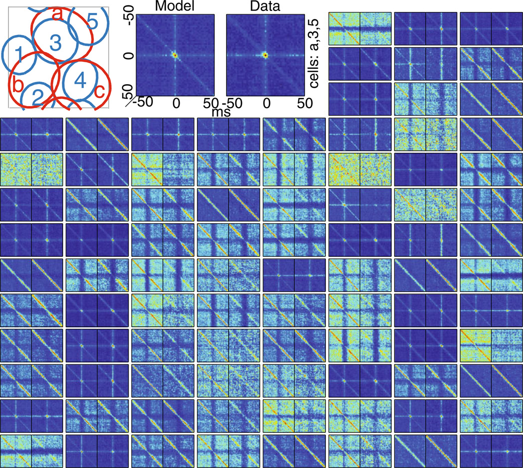
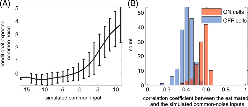
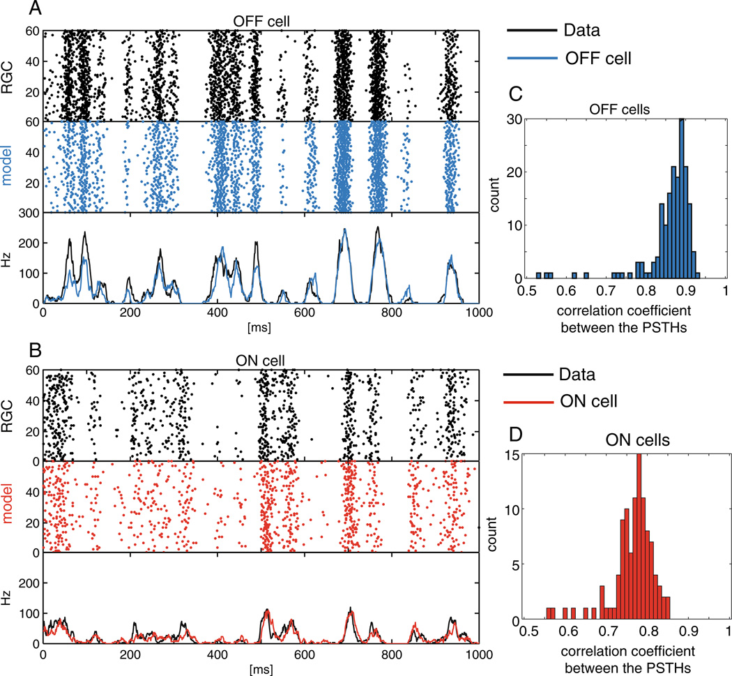
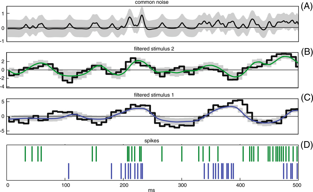
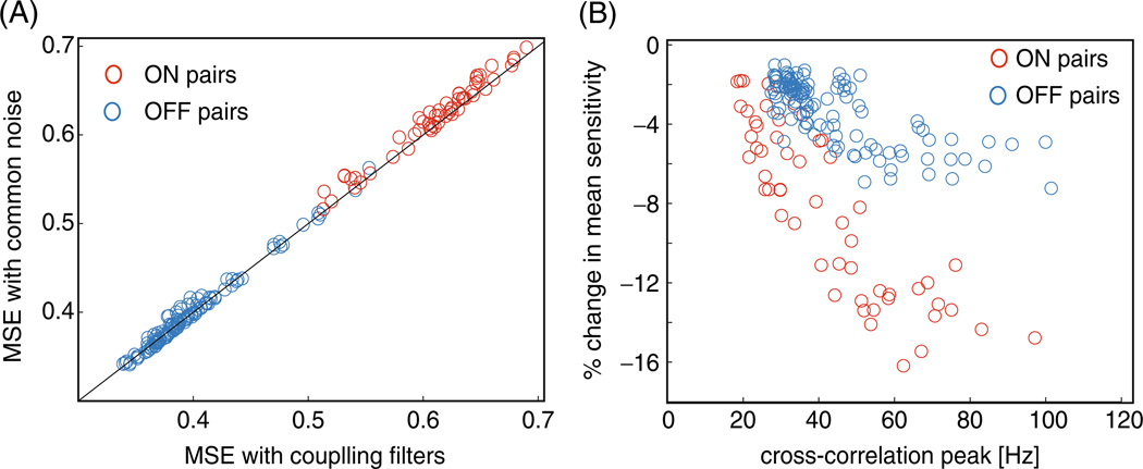
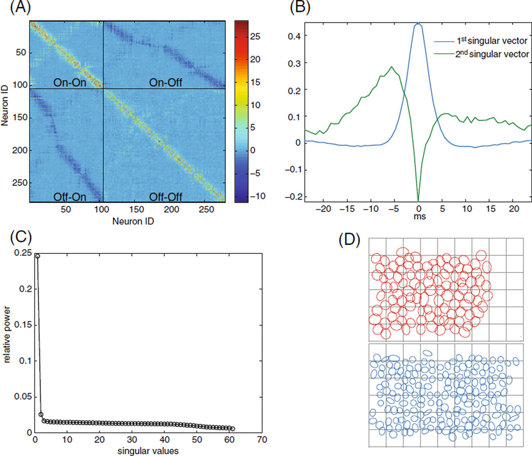
Synchronized spontaneous firing among retinal ganglion cells (RGCs), on timescales faster than visual responses, has been reported in many studies. Two candidate mechanisms of synchronized firing include direct coupling and shared noisy inputs. In neighboring parasol cells of primate retina, which exhibit rapid synchronized firing that has been studied extensively, recent experimental work indicates that direct electrical or synaptic coupling is weak, but shared synaptic input in the absence of modulated stimuli is strong. However, previous modeling efforts have not accounted for this aspect of firing in the parasol cell population. Here we develop a new model that incorporates the effects of common noise, and apply it to analyze the light responses and synchronized firing of a large, densely-sampled network of over 250 simultaneously recorded parasol cells. We use a generalized linear model in which the spike rate in each cell is determined by the linear combination of the spatio-temporally filtered visual input, the temporally filtered prior spikes of that cell, and unobserved sources representing common noise. The model accurately captures the statistical structure of the spike trains and the encoding of the visual stimulus, without the direct coupling assumption present in previous modeling work. Finally, we examined the problem of decoding the visual stimulus from the spike train given the estimated parameters. The common-noise model produces Bayesian decoding performance as accurate as that of a model with direct coupling, but with significantly more robustness to spike timing perturbations.

Fig. 1

Model schemas. (A) Fully general model. Each cell is modeled independently using a Generalized Linear model augmented with a state-space model (GLSSM). The inputs to the cell are: stimulus convolved with a linear spatio-temporal filter (kⁱ · x_t in Eq. (1)), past spiking activity convolved with a history filter ( ${\mathbf{h}}^i·{\mathbf{y}}_t^i$ ), past spiking activity of all other cells convolved with corresponding cross-coupling filters ( ${\displaystyle {\sum }_{j\ne i}^{n_{\text{cells}}}{\mathbf{L}}_{i,j}}·{\mathbf{y}}_t^j$ ), and a mixing matrix, M, that connects n_q common noise inputs $q_t^r$ to the n_cells observed RGCs. (B) Pairwise model. We simplify the model by considering pairs of neurons separately. Therefore, we have two cells and just one shared common noise. (C) Common-noise model where we set all the cross-coupling filters to zero and have n_cells independent common-noise sources coupled to the RGC network via the mixing matrix M

Fig. 2

Relative contribution of self post-spike, stimulus inputs, cross-coupling inputs, and common noise inputs to a pair of ON cells. In panels (A) through (D) blue indicates cell 1 and green cell 2. Panel (A): The observed spike train of these cells during this second of observation. Panel (B): Estimated refractory input from the cell, ${\mathbf{h}}^i·{\mathbf{y}}_t^i$ . In panels B through D the traces are obtained by convolving the estimated filters with the observed spike-trains. Panel (C): The stimulus input, kⁱ · x_t. Panel (D): Estimated cross-coupling input to the cells, ${\mathbf{L}}_{i,j}·{\mathbf{y}}_t^j$ . Panel (E): MAP estimate of the common noise, q̂_t (black), with one standard deviation band (gray). Red trace indicates a sample from the posterior distribution of the common noise given the observed data. Note that the cross-coupling input to the cells are much smaller than all other three inputs to the cell. Panel (F): The cross-correlations of the two spike trains (black - true spike trains, red-simulated spike trains). Panel (G): The three point correlations function of the common-noise and the spike trains, C(τ₁, τ₂) = [〈q(t)y₁(t + τ₁)y₂(t + τ₂)〉 − 〈q(t)〉〈y₁(t)〉 〈y₂(t)〉]/(〈y₁(t)〉〈y₂(t)〉dt). Note that when the two cells fire in synchrony the common-noise tends to be high (as can be seen from the warm colors at the center of the figure)

Fig. 3

Population summary of the inferred strength of the inputs to the model. (A) Summary plot of the relative contribution of the common noise (circles) and cross-coupling inputs (crosses) to the cells as a function of the cells’ distance from each other in the pairwise model for the complete network of 27 cells. Note that the common noise is stronger then the cross-coupling input in the large majority of the cell pairs. Since the OFF cells have a higher spike rate on average, the OFF–OFF cross-coupling inputs have a larger contribution on average than the ON–ON cross-coupling inputs. However, the filter magnitudes agree with the results of Trong and Rieke (2008); the cross-coupling filters between ON cells are stronger, on average, than the cross-coupling filters between OFF cells (not shown). The gap under 100 µm is due to the fact that RGCs of the same type have minimal overlap (Gauthier et al. 2009). (B) Histograms showing the relative magnitude of the common noise and stimulus plus post-spike filter induced inputs to each cell under the common-noise model. The X-axis is the ratio of the RMS of each of these inputs $\left(\sqrt{\frac{\mathit{\text{var}}({\hat{q}}_t)}{\mathit{\text{var}}({\mathbf{h}}^i·{\mathbf{y}}_t^i+{\mathbf{k}}^i·{\mathbf{x}}_t)}}\right)$ . Common inputs tend to be a bit more than half as strong as the stimulus and post-spike inputs combined

Fig. 4

Comparing the inferred common noise strength (right) and the receptive field overlap (left) across all ON–ON and OFF–OFF pairs. Note that these two variables are strongly dependent; Spearman rank correlation coefficent = 0.75 (computed on all pairs with a positive overlap, excluding the diagonal elements of the displayed matrices). Thus the strength of the common noise between any two cells can be predicted accurately given the degree to which the cells have overlapping receptive fields. The receptive field overlap was computed as the correlation coefficient of the spatial receptive fields of the two cells; the common noise strength was computed as the correlation value derived from the estimated common noise spatial covariance matrix C_s (i.e., C_s(i, j)/ $\sqrt{{\mathbf{C}}_s(i,i){\mathbf{C}}_s(j,j)}$ ). Both of these quantities take values between −1 and 1; all matrices are plotted on the same color scale

Fig. 5

Comparing real versus predicted cross-correlations. Example of 48 randomly selected cross-correlation functions of retinal responses and simulated responses of the common-noise model without direct cross-coupling (Fig. 1(C)). Each group of three panels shows the cross-correlation between a randomly selected reference ON/OFF (red/blue) cell and its three nearest neighbor cells (see schematic receptive field inset and enlarged example). In black is the data, in blue/red is the generated data using the common input model, and in green is the data generated with the common input turned off. The baseline firing rates are subtracted; also, recall that cells whose firing rate was too low or which displayed spike-sorting artifacts were excluded from this analysis. Each cross-correlation is plotted for delays between −96 to 96 ms. The Y-axis in each plot is rescaled to maximize visibility. The cross correlation between cells of the same type is always positive while opposite type cells are negatively cross correlated. Therefore, a blue positive cross correlation indicates an OFF–OFF pair, a red positive cross correlation indicates an ON–ON pair, and a blue/red negative cross-correlation indicates a OFF–ON/ON–OFF pair. Note that the cross-correlation at zero lag is captured by the common noise

Fig. 6

Comparing real and predicted triplet correlations. 89 example third-order (triplet) correlation functions between a reference cell (a in the schematic receptive field) and its two nearest-neighbors (cells 3 and 5 in the schematic receptive field). Triplet correlations were computed in 4-ms bins according to C(τ₁, τ₂) = [〈y₁(t)y₂(t + τ₁)y₃(t + τ₂)〉 − 〈y₁(t)〉〈y₂(t)〉 〈y₃(t)〉]/(〈y₂(t)〉〈y₃(t)〉dt). Color indicates the instantaneous spike rate (in 4 ms bins) as a function of the relative spike time in the two nearest neighbor cells for time delays between −50 to 50 ms. The left figure in each pair is the model (Fig. 1(C)) and the right is data. The color map for each of the two plots in each pair is the same. For different pairs, the color map is renormalized so that the maximum value of the pair is red. Note the model reproduces both the long time scale correlations and the peaks at the center corresponding to short time scale correlations

Fig. 7

Comparing simulated and inferred common-noise effects given the full population spike train. (A) The conditional expected inferred common-noise input q̂, averaged over all cells in the population, ± 1 s.d., versus the simulated common-noise input q. Note that the estimated input can be approximated as a rectified and shrunk linear function of the true input. (B) Population summary of the correlation coefficient between the estimated common-noise input and the simulated common-noise input for the entire population

Fig. 8

Comparing real versus predicted PSTHs. Example raster of responses and PSTHs of recorded data and model-generated spike trains to 60 repeats of a novel 1 sec stimulus. (A) OFF RGC (black) and model cell (blue). (B) ON RGC (black) and model ON cell (red). (C)–(D) Correlation coefficient between the model PSTHs and the recorded PSTHs for all OFF (C) and ON cells (D). The model achieves high accuracy in predicting the PSTHs

Fig. 9

Stimulus decoding given a pair of spike trains. In panels (B) through (D) blue indicates cell 1 and green cell 2. (A) MAP estimate of the common noise going into two cells (black) with one standard deviation of the estimate (gray). (B) and (C) panels: The true stimulus filtered by the estimated spatio-temporal filter trace, kⁱ · x_t, (black) and the MAP estimate of the filtered stimulus (green/blue) with one standard deviation (gray). Decoding performed following the method described in Section 2.4. (D) The spike trains of the two cells used to perform the decoding

Fig. 10

Decoding jitter analysis. (A) Without any spike jitter, the two models decode the stimulus with nearly identical accuracy. Each point represents the decoding performance of the two models for a pair of cells. In red: ON–ON pairs. In blue: OFF–OFF. (B) Jitter analysis of the common noise model versus the direct coupling model from Pillow et al. (2008). The X axis denotes the maximum of the cross-correlation function between the neuron pair. Baseline is subtracted so that units are in spikes/s above (or below) the cells’ mean rate. The Y axis is the percent change ( $\frac{S_{\mathit{\text{common}}-\mathit{\text{noise}}}-S_{\mathit{\text{direct}}-\mathit{\text{coupling}}}}{S_{\mathit{\text{common}}-\mathit{\text{noise}}}}*100$ ) in the model’s sensitivity to jitter ( $S=\frac{\sqrt{{\mathbf{U}}_{\mathit{\text{jitter}}}-\mathbf{U}}}{|\mathrm{\Delta }t|}$ ) compared to the change in sensitivity of the direct coupling model: negative values mean that the common noise model is less sensitive to jitter than a model with direct cross-coupling. Note that the common-noise model leads to more robust decoding in every cell pair examined, and pairs that are strongly synchronized are much less sensitive to spike-train jitter in the common noise model than in the model with coupling filters

Fig. 11

PSTH-based method (A) Approximate spatial covariance matrix of the inferred common noise composed of the first two spatial singular vectors. ${\tilde{C}}_{i,j}={\displaystyle {\sum }_{k=1}^2{\sigma }_k{U}_k}$ (the vectors are reshaped into matrix form). Note the four distinct regions corresponding to the ON–ON, OFF–OFF, ON–OFF, and OFF–ON. (B) First two temporal singular vectors, corresponding to the temporal correlations of the ‘same-type’ (ON–ON and OFF–OFF pairs), and ‘different type’(ON–OFF pairs). Note the asymmetry of the ON–OFF temporal correlations. (C) Relative power of all the singular values. Note that the first two singular values are well separated from the rest, indicating the correlation structure is well approximated by the first two singular vectors. (D) Receptive field centers and the numbering schema. Top in red: ON cells. Bottom in blue: OFF cells. The numbering schema starts at the top left corner and goes column-wise to the right. The ON cells are 1 through 104 and the OFF cells are 105 to 277. As a result, cells that are physically close are usually closely numbered

References

1. Agresti A. Wiley series in probability and mathematical statistics. 2002. Categorical data analysis.
1. Ahmadian Y, Pillow J, Shlens J, Chichilnisky E, Simoncelli E, Paninski L. COSYNE09. 2009. A decoder-based spike trainmetric for analyzing the neural code in the retina.
1. Ahmadian Y, Pillow JW, Paninski L. Efficient Markov chain Monte Carlo methods for decoding neural spike trains. Neural Computation. 2011;23:46–96. - PMC - PubMed
1. Arnett D. Statistical dependence between neighboring retinal ganglion cells in goldfish. Experimental Brain Research. 1978;32(1):49–53. - PubMed
1. Bickel P, Doksum K. Mathematical statistics: Basic ideas and selected topics. Prentice Hall; 2001.
Publication types
LinkOut - more resources