An overview of longitudinal data analysis methods for neurological research

Abstract

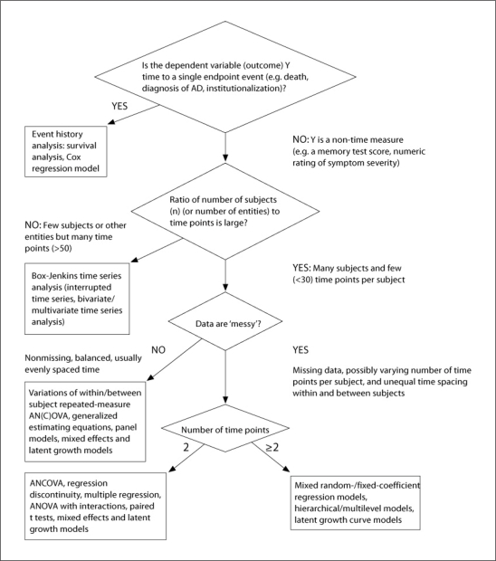
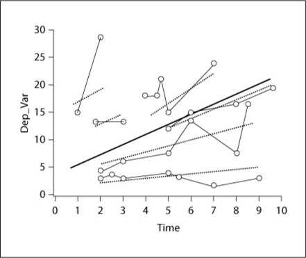
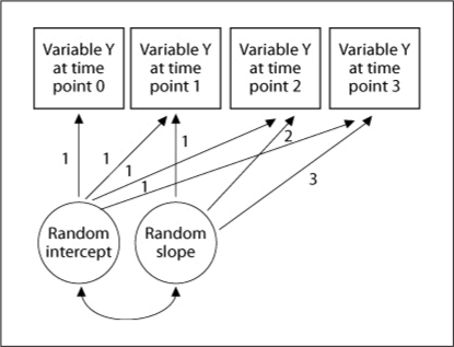
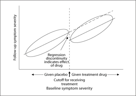
The purpose of this article is to provide a concise, broad and readily accessible overview of longitudinal data analysis methods, aimed to be a practical guide for clinical investigators in neurology. In general, we advise that older, traditional methods, including (1) simple regression of the dependent variable on a time measure, (2) analyzing a single summary subject level number that indexes changes for each subject and (3) a general linear model approach with a fixed-subject effect, should be reserved for quick, simple or preliminary analyses. We advocate the general use of mixed-random and fixed-effect regression models for analyses of most longitudinal clinical studies. Under restrictive situations or to provide validation, we recommend: (1) repeated-measure analysis of covariance (ANCOVA), (2) ANCOVA for two time points, (3) generalized estimating equations and (4) latent growth curve/structural equation models.

Keywords: Analysis; Longitudinal studies; Methods; Neurology; Statistics.

Fig. 1

a A ‘spaghetti plot’ of raw longitudinal data (example from Dodd et al. [28]). Raw BDS vs. years in study for 493 AD patients, each having 3–14 observations over time (years in study). The BDS score is the number of errors made on a measure of cognition (higher score means the patient is performing worse). Thin lines connect scores for an individual person. The thick straight solid line is the OLS regression line, and the thick dashed line is the OLS quadratic curve (this graph was produced with SAS Graph software, Proc Gplot). b The same data after removal of the pure time or visit level random error via a random-effect model, leaving subject level random quadratic and linear time terms and fixed effects. c The same data after additionally removing the subject level random quadratic and linear effects, leaving only fixed effects which included an interaction between baseline level of the BDS and a quadratic effect of time, shown in the figure as a predicted accelerating increase for subjects with low baseline levels but a decelerating increase for those with high baseline levels.

Fig. 2

a Illustrative mean ADL values vs. years in study, predicted by best-fitting longitudinal mixed-effect model for 382 AD patients treated with various medication regimens and starting at different initial mean ADL values (0, 25, 50). Score = Dependency (%) on other people; square = no medication; × = cholinesterase inhibitors only; dot = combination of cholinesterase inhibitors and memantine. Baseline ADL values and their linear/nonlinear interaction with time were included as fixed predictors. Note the differing trajectories depending on the baseline level, and superimposed on that is a medication group effect whereby the combination therapy apparently dampens clinical progression as measured by the ADL (from Atri et al. [29]). b Illustrative mean BDS scores across time predicted by the fitted mixed model in the longitudinal analysis for log plasma CRP for 122 AD patients, for selected levels of baseline log CRP and example time span. Illustrative levels of log CRP were chosen to correspond to the 1st, 25th, 50th (median), 75th and 99th percentiles of its distribution (from Locascio et al. [30]).

Fig. 3

Fitting sigmoid data with a cubic model. Data were created to approximate a sigmoid shape with a floor, ceiling, and some normally distributed random error (error std. dev. = 2). Best-fitting cubic and logistic curves are shown. Note the cubic curve bends slightly at tails in contrast to the logistic curve, a difference which may be trivial or unacceptable depending on the situation. The cubic function accounted for 95.2% of the variance in the dependent variable, and the logistic model accounted for 95.4%.

Fig. 4

Flow chart for deciding which method to use to analyze longitudinal data (with continuous numeric outcome) in neurological research. This flow chart should be considered only a rough guide; not all possible situations, exceptions, and combinations or variations of methods could be included.

Fig. 5

Illustration of a random-effect model. Simple, simulated longitudinal data illustrate what a mixed-fixed and random-coefficient model does in the case of a simple linear model. Values on the dependent variable (Dep_Var) are indicated by circles with a thin solid line connecting scores for the same subject. The thick solid line in the middle is the estimated overall group regression line (a ‘fixed’ term). The dotted straight lines are the regression lines with random slopes and intercepts fit to the subjects’ data, respectively. Note that when a subject has only a few observations, like the subject at the upper left, the slope and intercept of his regression line is weighted to be similar to the overall group average, whereas when a subject has relatively many observations, like the subject at the bottom of the graph, the regression line is more weighted in accordance to that subject's own values.

Fig. 6

A simple LGCM illustrated as SEM. Circles denote latent random variables, squares are observed measures, straight arrows are predictive effects, and the double-headed curved arrow denotes a possible correlation between the random intercept and random slope latent variables. Numbers are coefficients applied to the predictors (intercept and slope). (Measurement error terms pointing at each observed measure are not shown for simplicity.)

Fig. 7

Regression discontinuity design (ANCOVA) – illustrative example. Ellipses denote swarms of data points for two respective groups (e.g., medication-treated and placebo groups) in a scatterplot of follow-up symptom severity versus baseline symptom severity scores (higher numbers = more severe). Solid diagonal lines are regression lines for the groups. Here the slope of the regression lines, and orientation and shape of the ellipses indicate an expected strongly positive correlation of follow-up symptom severity to baseline symptom severity within each group. For ethical reasons, the medication treatment is given to anyone above a cutoff on symptom severity at baseline (this may especially be the case if the treatment is in limited supply or very expensive). (Perhaps the treatment, if shown effective, might be given to the placebo group at a later time.) Note the treated group has worse mean symptoms than the placebo group at baseline as well as at follow-up. However, the discontinuous drop in the regression line in moving from the placebo to the treated group strongly suggests a beneficial effect of the treatment which, if strong enough, would be reflected in a significant group effect on follow-up symptom severity in ANCOVA with the baseline symptom severity as the linear covariate.

References

1. SAS/Stat User's Guide, version 9.2. Cary: SAS Institute; 2011.
1. Mplus Statistical Software. Los Angeles: Muthen & Muthen; 2011.
1. SPSS Software. Chicago, Illinois: SPSS; 2011.
1. JMP Software. Cary: SAS; 2011.
1. Zeger SL, Liang KY. An overview of methods for the analysis of longitudinal data. Stat Med. 1992;11:1825–1839. - PubMed