Reducing system noise in copy number data using principal components of self-self hybridizations

Abstract

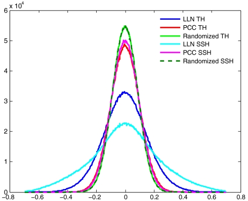
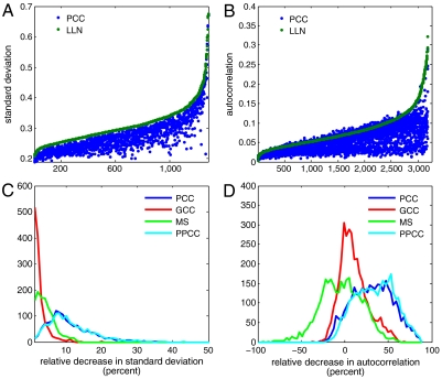
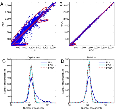
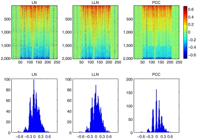
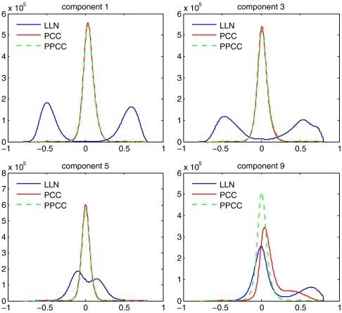
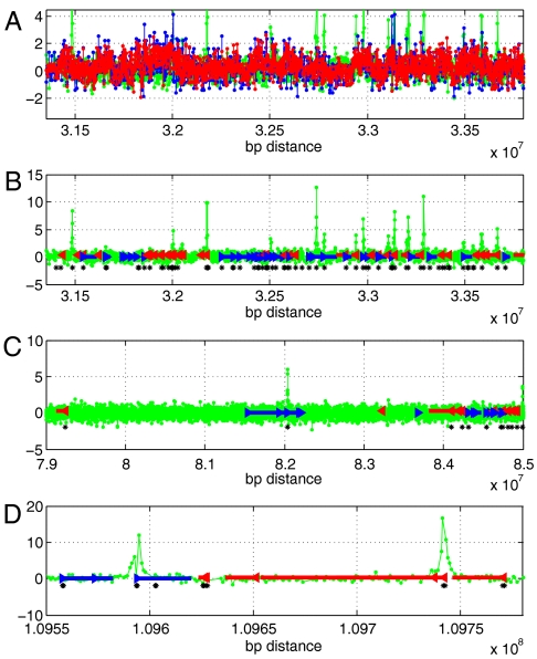
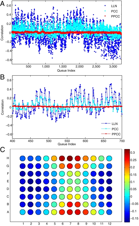
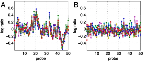
Genomic copy number variation underlies genetic disorders such as autism, schizophrenia, and congenital heart disease. Copy number variations are commonly detected by array based comparative genomic hybridization of sample to reference DNAs, but probe and operational variables combine to create correlated system noise that degrades detection of genetic events. To correct for this we have explored hybridizations in which no genetic signal is expected, namely "self-self" hybridizations (SSH) comparing DNAs from the same genome. We show that SSH trap a variety of correlated system noise present also in sample-reference (test) data. Through singular value decomposition of SSH, we are able to determine the principal components (PCs) of this noise. The PCs themselves offer deep insights into the sources of noise, and facilitate detection of artifacts. We present evidence that linear and piecewise linear correction of test data with the PCs does not introduce detectable spurious signal, yet improves signal-to-noise metrics, reduces false positives, and facilitates copy number determination.

Fig. 1.

Correction of long-range correlations in probe ratios. A random set of 2,000 probes with nonredundant mappings to the reference genome (hg18 build) was selected. From these, two 2,000 X 132 matrices of log ratios were created: one for 132 SSH and another for 132 randomly selected TH. Pearson correlations between matrix rows were computed before LLN and after applying PCC. The histogram also shows the distribution of correlations for LLN matrixes with independent random permutation of values within rows. The bin size for the histogram is 0.003.

Fig. 2.

Comparison of PCC to other normalization schemes. (A) The standard deviation of log ratios for “quiet autosomal probes” of 1,349 female hybridization were scaled by the mean values of stable X chromosome regions before (green) and after (blue) noise correction, sorted by increasing standard deviation before PCC. (B) Autocorrelation was calculated for the log ratios of these probes from 3,252 hybridizations before (green) and after (blue) PCC, again sorted by increasing autocorrelation before correction. (C) Histograms for relative percent decrease of standard deviation for four different noise corrections: PCC, GCC, MS, or PPCC. The bin size is 1% decrease. (D) Histograms for relative percent gain/loss of autocorrelation of “quiet probes” for four different noise corrections: PCC, GCC, MS, and PPCC. (PPCC refers to piecewise principal component correction; MS and PPCC are described in detail in the Materials and Methods.) In this panel, the bin size is 3%. Quiet probes are defined as autosomal probes for which the frequency of amplifications and deletions combined does not exceed 1% within the population. Amplifications and deletions are defined here as segments exceeding ± log(1.1). Relative percent gain/loss for quantity X is defined as (100^∗(X_before - X_after)/X_before)%, where X_before is the value after Lowess and local normalization (LLN).

Fig. 3.

Comparison of normalization methods in sample-reference hybridizations. Data for probes on all autosomes, before and after PCC or PPCC, were segmented from 3,252 hybridizations, median segmented ratio values assigned to each probe, and values above a 1.1 ratio threshold were counted. (A) Amplification count, with LLN (X axis) vs. PCC (Y axis). Circled region A represents a large set of segments detected before PCC, which are mostly not detected as segments after PCC; circled region B indicates a subset of very common copy number polymorphisms that are detected somewhat less frequently following PCC. Circled region C shows the common copy number polymorphisms that are detected more frequently following PCC. (B) Same as (A), except PCC (X axis) is compared to PPCC (Y axis). The circled region represents a small set of probes that are less frequently segmented for which the correction is improved. (C, D) Histograms of the number of segments with mean ratio value exceeding 1.1 (duplications) and less than 1/1.1 in ratio mean value (deletions). Bin size for number of segments is fixed in logarithmic scale.

Fig. 4.

Discrete copy number states at a commonly polymorphic site after PCC. The selected region (chr7:143504894-143707170, hg18 build) consists of a CNV locus (encompassing 170 probes) with 40 nonpolymorphic flanking probes on each side (X axis). Upper: the log ratio values of 2,028 hybridizations (Y axis) for all probes in the extended region are shown, for which rows are sorted in descending order by segment median ratios within the CNV. Lower: histograms of segment median ratios corresponding to the panels directly above. Following local normalization (Left) and LLN (Middle), varying copy number states are only moderately evident. PCC (Right) resolves at least six distinct states at this locus.

Fig. 5.

Extent of probe correction following PCC and PPCC. For each of 14 components, a matrix of log ratios was created, consisting of 1,500 columns, one for each hybridizations of the parents, with about 4,200 rows, and one for each probe with extreme loadings (most positive and negative 0.1% of values). Pearson correlations were computed between all pairs of rows. Histograms of these correlations are shown for components 1, 3, 5, and 9, before and after PCC or PPCC. (Fig. S1 shows histograms for all principal components.) The bin size for the histograms is 0.005.

Fig. 6.

Loadings from components 1 and 9 in genome order, in relation to G + C nucleotide content and gene transcription units. (A) We examined the scaled (by 10³) loadings of components 1 (red) and 9 (green) in genome order from a representative gene-rich region. The blue is the C + G content of each probe (shifted and scaled), showing the rough overlap of the loadings of component 1 and the C + G content of the probes. (B) The coincidence of peaks of loadings in component 9 is illustrated with respect to genes in the same region. Green lines indicate loadings of component 9; blue and red represent forward- and reverse-strand genes, respectively; and the arrows indicate the direction of transcription and gene boundaries. Black asterisks show the genomic positions of CpG islands. (C, D) The same relationships shown in (B) are displayed in different regions and at different scales. Probes with high loading from the ninth component are clustered about the 5′ ends of genes, especially genes with nearby CpG islands. All information is derived from the hg18 build and UCSC Genome Browser (http://genome.ucsc.edu/) with coordinates on chromosome 1 as indicated on the X-axis.

Fig. 7.

Correlation of component 9 with microwell sample coordinates. Variation in correlation of component 9 with extreme (1.5% most positive and negative) probes over 3252 hybridizations has a periodicity of 12 with respect to the queue index (A and B), before (LLN) and after PCC, but not after PPCC. For (C), correlations computed for LLN data were adjusted in each 96-well plate to have a mean of zero and a standard deviation of 1. The adjusted values were then averaged over the same row and column coordinates from the 41 8-by-12 microwell plates in which the samples used for the hybridizations were stored and shipped. These values are displayed in microwell coordinates, with red for highly positive and blue for highly negative correlations.

Fig. P1.

Correction of trends in copy number data using the principal components of self-self hybridization. To illustrate the problem and solution, we selected one region of 50 contiguous probes and displayed the log ratio from various hybridizations. (A) shows ten self-self hybridizations, in which coherent trends are evident. (B) shows the corresponding log ratio data from the same region after principal component correction.

References

1. Iafrate AJ, et al. Detection of large-scale variation in the human genome. Nat Genet. 2004;36:949–951. - PubMed
1. Sebat J, et al. Large-scale copy number polymorphism in the human genome. Science. 2004;305:525–528. - PubMed
1. Nei M, Niimura Y, Nozawa M. The evolution of animal chemosensory receptor gene repertoires: Roles of chance and necessity. Nat Rev Genet. 2008;9:951–963. - PubMed
1. Perry GH, et al. Diet and the evolution of human amylase gene copy number variation. Nat Genet. 2007;39:1256–1260. - PMC - PubMed
1. Stankiewicz P, Lupski JR. Structural variation in the human genome and its role in disease. Annu Rev Med. 2010;61:437–455. - PubMed
Publication types
Associated data