Phase-amplitude coupling in human electrocorticography is spatially distributed and phase diverse

Abstract

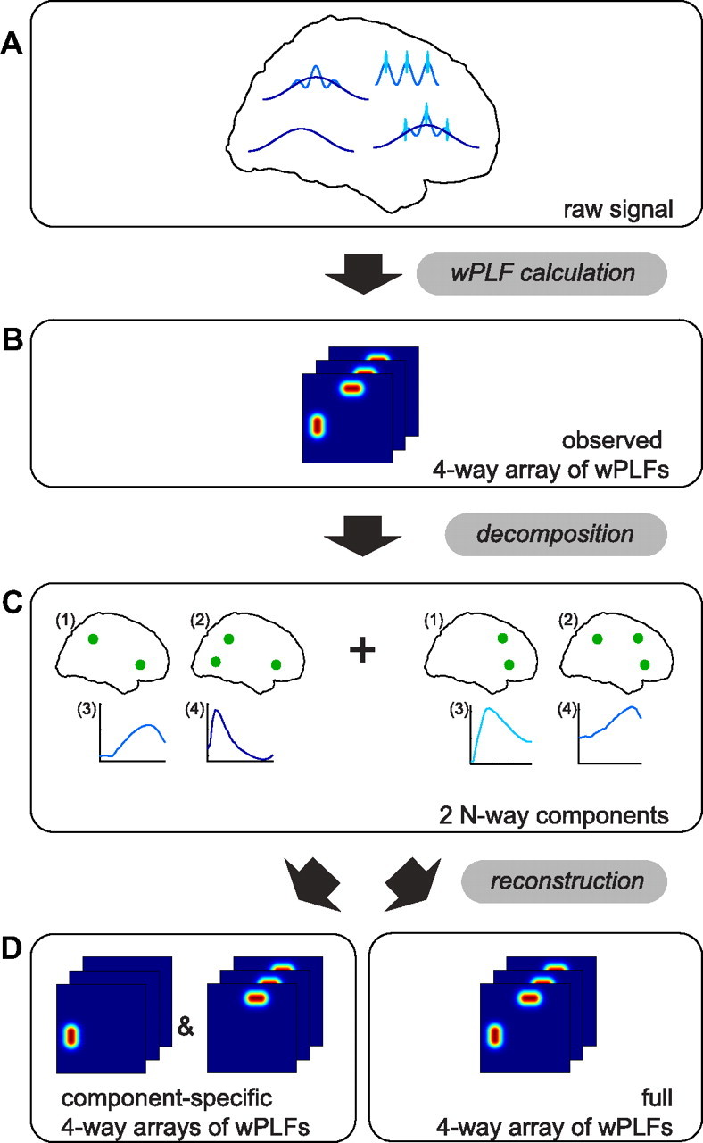
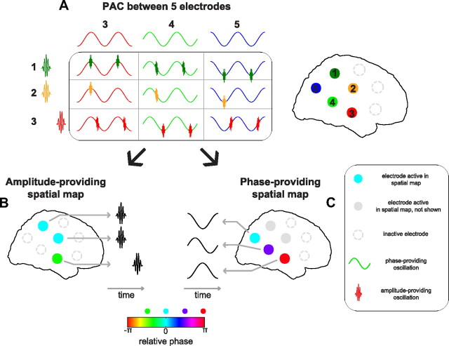
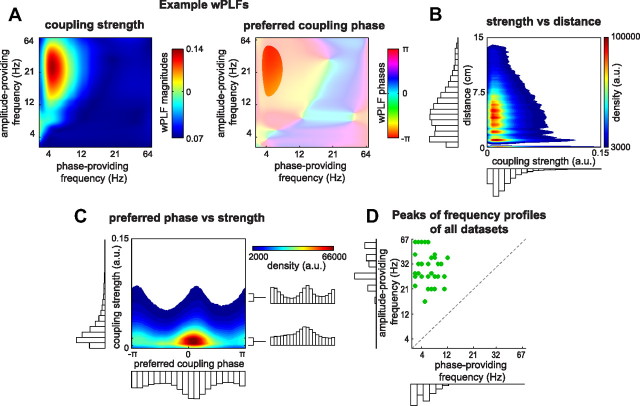
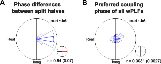
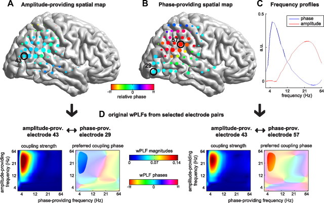
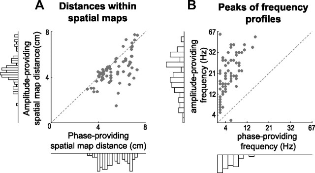
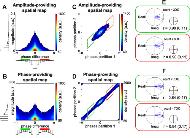
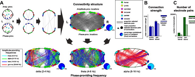
Spatially distributed phase-amplitude coupling (PAC) is a possible mechanism for selectively routing information through neuronal networks. If so, two key properties determine its selectivity and flexibility, phase diversity over space, and frequency diversity. To investigate these issues, we analyzed 42 human electrocorticographic recordings from 27 patients performing a working memory task. We demonstrate that (1) spatially distributed PAC occurred at distances >10 cm, (2) involved diverse preferred coupling phases, and (3) involved diverse frequencies. Using a novel technique [N-way decomposition based on the PARAFAC (for Parallel Factor analysis) model], we demonstrate that (4) these diverse phases originated mainly from the phase-providing oscillations. With these properties, PAC can be the backbone of a mechanism that is able to separate spatially distributed networks operating in parallel.

Figure 1.

Schematic representation of analyses. The data flow in our analyses is illustrated by a schematic decomposition and reconstruction of two different PAC patterns, one between a slow and a medium fast rhythm, and one between the medium fast and a very fast rhythm. These two PAC patterns have a different spatial distribution. After calculating a 4-way array of wPLFs, the two PAC patterns are separated in two different components using our N-way decomposition. The two patterns can then be reconstructed individually into two 4-way arrays of wPLFs or jointly into one 4-way array of wPLFs. For the purpose of simplicity, we have left out phase information in this schematic. Phase information is crucial throughout our analyses and is important for separating PAC patterns. A, PAC at four electrodes involving three oscillations. Not all oscillations are present at each location. B, 4-way array of wPLFs obtained from the raw data in A. The dimensions of this 4-way array are (1) amplitude-providing electrodes, (2) phase-providing electrodes, (3) amplitude-providing frequencies, and (4) phase-providing frequencies. C, Decomposition of the 4-way array of wPLFs in B into two components. Each component describes one PAC pattern, and each consists of an (1) amplitude-providing spatial map, a (2) phase-providing spatial map, an (3) amplitude-providing frequency profile, and a (4) phase-providing frequency profile. D, Reconstruction of 4-way arrays of wPLFs based on the decomposition in C. On the left, we show the component-specific reconstruction, in which each component is used to create one 4-way array of wPLFs, which is determined by only one PAC pattern. On the right, we show the full reconstruction, resulting in a 4-way array of wPLFs describing both PAC patterns. For details, see Materials and Methods.

Figure 2.

Preferred coupling phases in spatially distributed PAC are decomposed into relative phases in amplitude- and phase-providing spatial maps. Phase diversity of PAC is fully explained by the two complex-valued spatial maps (i.e., phase variability over space). A, Schematic representation of PAC between five electrodes. B, Schematic amplitude-providing spatial map with three electrodes that show amplitude bursts. Color indicates the relative phase of the electrodes. The third electrode has a phase shift of π/2 relative to the other electrodes. This reflects a time offset of the corresponding amplitude-providing oscillation, given by the phase offset and the cycle length of the phase-providing oscillation in C. C, Same as B but for the phase-providing spatial map. The phase-providing oscillations have a phase offset equal to their relative phases. Note that we cannot distinguish between the case in which every cycle of the phase-providing oscillation has a burst of the amplitude-providing oscillation (first row of table) and the case in which only some cycles of the phase-providing oscillation have a burst (second row of table).

Figure 3.

PAC occurred over long distances, has diverse preferred coupling phases, and involved many frequencies. A, Example wPLFs for one electrode pair. For this electrode pair, the strongest coupling is between the phase of a theta oscillation (∼3–8 Hz) and the amplitude of a beta/gamma oscillation (∼18–42 Hz). The preferred coupling phase is π, which corresponds to the trough of the theta oscillation. Color bar codes reflect wPLF magnitude and phase. B, Density of the significant wPLFs from all datasets as a function of their strength and the distance between the amplitude- and phase-providing electrodes. The majority of PAC occurs at distances ∼6 cm and can go up to ∼14 cm. Color bar code reflects the density of wPLFs at each X–Y coordinate. C, Density of the significant wPLFs as a function of their preferred coupling phase and their strength. PAC occurs with diverse preferred coupling phase, with most preferred phases around the peak of the phase-providing oscillation (angle = 0). However, especially for the wPLFs that show a strong coupling, preferred phases also cluster at the trough (angle = ±π). Color bar code same as in B. D, Scatter plot of the peaks of the frequency profiles obtained from the significant wPLFs (see Materials and Methods). The peak phase-providing frequencies show a substantial spread, ranging from delta to alpha, and so do the amplitude-providing frequencies, ranging from beta to gamma.

Figure 4.

Diversity in preferred coupling phase is produced by reliable phase estimates. To estimate the reliability of our phase estimates, we randomly partitioned the trials of each dataset into two sets. A 4-way array of wPLFs was then calculated for each of the two sets of trials. A, Histogram of phase differences between wPLFs of the first and the second set of trials for all datasets. The majority of phase differences are very close to 0, indicating that the preferred coupling phases are highly similar in the two sets of trials. The reliability coefficient, calculated on these phase differences (see Materials and Methods), was on average 0.84 ± 0.07 (SD). B, For comparison with the reliability results in A, we show the same information for the preferred coupling phase of the wPLFs, instead of their between-set phase differences. The phase histogram shows diversity in preferred coupling phase (same information as in Fig. 3C). We calculated the same coefficient as in A but now applied to the preferred coupling phase (instead of the between-set phase differences) and found that it was on average 0.0031 ± 0.0027 (SD). The difference with the average reliability coefficient shows that our phase estimates are highly reliable.

Figure 5.

N-way decomposition reveals the spatial distribution in PAC in sets of two spatial maps and two frequency profiles. Each 4-way array of wPLFs from each dataset was decomposed into one or more components, each component being a set of two spatial maps and two frequency profiles. The diversity in the preferred coupling phase is explained by the two complex-valued spatial maps, namely by their phase diversity across space. A–C, Example component from a representative subject. A, Amplitude-providing spatial map. B, Phase-providing spatial map. Both the amplitude- and phase-providing spatial map are widely distributed over the cortex, but the phase-providing spatial map is wider and shows more phase diversity. The size of the markers indicates the contribution of each electrode to the spatial map, and the color indicates the relative phase of the electrodes. C, Amplitude- and phase-providing frequency profiles. These profiles show that the example component involves a coupling between the phase of a theta oscillation and the amplitude of a beta/gamma oscillation. D, wPLFs (for all frequency pairs) of two selected electrode pairs. The frequency pairs for which there is strong coupling closely match the frequency profiles in C, and the difference between the preferred coupling phases closely match the corresponding phase difference in the phase-providing spatial map.

Figure 6.

Spatial extent of spatial maps and frequency profiles. A, Mean distance within components in phase-providing spatial maps (horizontal axis) plotted against the mean distance in amplitude-providing spatial maps (vertical axis). The mean distance within components was on average higher for the phase-providing than for the amplitude-providing spatial maps (paired samples t test; t₍₈₄₎ = −5.56, p < 1e-6). B, Scatter plot of the peaks of the phase-providing frequencies (horizontal axis) versus the peaks of the amplitude-providing frequencies (vertical axis). There is a substantial spread of the peaks of the phase-providing frequency profiles, ranging from delta to alpha, and those of the amplitude-providing frequency profiles, ranging from theta to gamma. Note the difference with respect to Figure 3D, and see Results for a possible explanation. For selection of electrodes, see Materials and Methods.

Figure 7.

Phase-providing and amplitude-providing spatial maps show different phase configurations. To investigate the phase configurations of both types of spatial maps, we computed the phase differences for all possible pairs of electrodes selected from a spatial map. A, Density of electrode pairs of each spatial map as a function of their magnitude and their phase differences for the amplitude-providing spatial map. Phase differences cluster around 0. B, Same as in A but for the phase-providing spatial map. Phase differences are mostly around 0 and ±π. C–F, To investigate the reliability of the phase differences, we evaluated the split-half reliability of our decomposition results (see Results and Materials and Methods). C, Density of amplitude-providing spatial map phase differences from the first versus those of the second set. D, Same information as in C but for phase-providing spatial maps. Between-set phase differences are highly similar for both spatial maps, showing that they are highly reliable. E, Phase histograms and mean resultant vector of the amplitude-providing spatial map between-set phase differences for the intervals from −2π/3 to −π/3 (green box) and from π/3 to 2π/3 (red box). F, Same as in E but for the phase-providing spatial maps. For both types of spatial maps, between-set phase differences cluster around 0, indicating reliability of the between-electrode phase differences in this narrow range. For a description of the reliability coefficient r, see Results. For selection of electrodes, see Materials and Methods.

Figure 8.

Differential connectivity structure in PAC components with different phase-providing frequencies. To investigate the connectivity structure in PAC, we aggregated over all pairs of selected electrodes from all 85 N-way components (for electrode selection, see Materials and Methods). The original Talairach-based locations were downsampled to 23 unique locations on both the left and the right hemisphere. Every resulting connection was indexed by the proportion of its electrode pairs that were selected. Note that not all possible connections were observed in the data (see Results). A, Connectograms. Schematic on the left depicts the construction of a connectogram for a set of connected electrodes. In all connectograms, line thickness indicates the proportion of selected electrode pairs within a downsampled connection (if a proportion is 0, the line is absent). Furthermore, node color indicates lobe, and node size indicates the sum of the proportions of selected electrode pairs of all its connections. Pie charts indicate the number of non-zero ipsilateral versus contralateral connections within a connectogram. The bottom three connectograms were obtained by splitting the connections according to their phase-providing frequency. In these connectograms, line color indicates the amplitude-providing frequency of the connection. Because of spatial downsampling, every connection represents many electrode pairs from multiple N-way components. The frequency color code was based on the mode of the distribution (over electrode pairs) of the associated peak frequency profiles. Components that differ in the frequency of their phase-providing oscillation have connectograms that differ greatly in their connectivity pattern, including their degree of cross-hemispheric lateralization. B, Mean of the contralateral versus ipsilateral and the within- versus between-lobe connection strengths. Means are taken over the median connection strength of the electrode pairs forming a connection. The connection strengths were computed by selecting their component-specific reconstructed wPLFs and taking a weighted average over the two frequency dimensions. C, Number of electrode pairs selected and observed for contralateral and ipsilateral connections.

References

1. Akam T, Kullmann DM. Oscillations and filtering networks support flexible routing of information. Neuron. 2010;67:308–320. - PMC - PubMed
1. Amzica F, Steriade M. The K-complex: its slow (<1-Hz) rhythmicity and relation to delta waves. Neurology. 1997;49:952–959. - PubMed
1. Axmacher N, Henseler MM, Jensen O, Weinreich I, Elger CE, Fell J. Cross-frequency coupling supports multi-item working memory in the human hippocampus. Proc Natl Acad Sci U S A. 2010;107:3228–3233. - PMC - PubMed
1. Beckmann CF, Smith SM. Tensorial extensions of independent component analysis for multisubject FMRI analysis. Neuroimage. 2005;25:294–311. - PubMed
1. Bro R. Models, algorithms, and applications. Amsterdam: University of Amsterdam; 1998. Multi-way analysis in the food industry.
Publication types
LinkOut - more resources