Probabilistic inference in general graphical models through sampling in stochastic networks of spiking neurons

Abstract

An important open problem of computational neuroscience is the generic organization of computations in networks of neurons in the brain. We show here through rigorous theoretical analysis that inherent stochastic features of spiking neurons, in combination with simple nonlinear computational operations in specific network motifs and dendritic arbors, enable networks of spiking neurons to carry out probabilistic inference through sampling in general graphical models. In particular, it enables them to carry out probabilistic inference in Bayesian networks with converging arrows ("explaining away") and with undirected loops, that occur in many real-world tasks. Ubiquitous stochastic features of networks of spiking neurons, such as trial-to-trial variability and spontaneous activity, are necessary ingredients of the underlying computational organization. We demonstrate through computer simulations that this approach can be scaled up to neural emulations of probabilistic inference in fairly large graphical models, yielding some of the most complex computations that have been carried out so far in networks of spiking neurons.

Figure 1. The visual perception experiment of that demonstrates “explaining away” and its corresponding Bayesian network model.

A) Two visual stimuli, each exhibiting the same luminance profile in the horizontal direction, differ only with regard to their contours, which suggest different 3D shapes (flat versus cylindrical). This in turn influences our perception of the reflectance of the two halves of each stimulus (a step in the reflectance at the middle line, versus uniform reflectance): the cylindrical 3D shape “explains away”the reflectance step. B) The Bayesian network that models this effect represents the probability distribution . 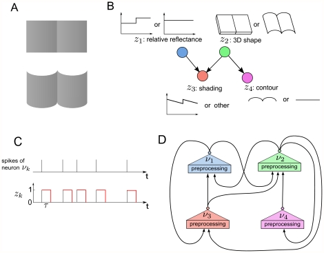The relative reflectance () of the two halves is either different ( = 1) or the same ( = 0). The perceived 3D shape can be cylindrical ( = 1) or flat ( = 0). The relative reflectance and the 3D shape are direct causes of the shading (luminance change) of the surfaces (), which can have the profile like in panel A ( = 1) or a different one ( = 0). The 3D shape of the surfaces causes different perceived contours, flat ( = 0) or cylindrical ( = 1). The observed variables (evidence) are the contour () and the shading (). Subjects infer the marginal posterior probability distributions of the relative reflectance and the 3D shape based on the evidence. C) The RVs are represented in our neural implementations by principal neurons . Each spike of sets the RV to 1 for a time period of length . D) The structure of a network of spiking neurons that performs probabilistic inference for the Bayesian network of panel B through sampling from conditionals of the underlying distribution. Each principal neuron employs preprocessing to satisfy the NCC, either by dendritic processing or by a preprocessing circuit.

Figure 2. Implementation 2 for the explaining away motif of the Bayesian network from Fig. 1B .

Implementation 2 is the neural implementation with auxiliary neurons, that uses the Markov blanket expansion of the log-odd ratio. There are 4 auxiliary neurons, one for each possible value assignment to the RVs and in the Markov blanket of . The principal neuron () connects to the auxiliary neuron directly if () has value 1 in the assignment , or via an inhibitory inter-neuron if () has value 0 in . The auxiliary neurons connect with a strong excitatory connection to the principal neuron , and drive it to fire whenever any one of them fires. The larger gray circle represents the lateral inhibition between the auxiliary neurons.

Figure 3. Results of Computer Simulation I.

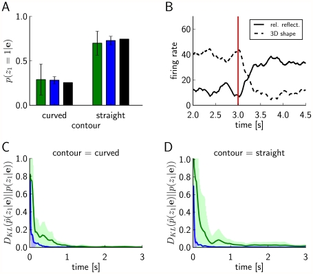
Performance comparison between an ideal version of Implementation 1 (use of auxiliary RVs, results shown in green) and an ideal version of implementations that satisfy the NCC (results shown in blue) for probabilistic inference in the Bayesian network of Fig. 1B (“explaining away”. Evidence (see (1)) is entered for the RVs and , and the marginal probability is estimated. A) Target values of for and are shown in black, results from sampling for from a network of spiking neurons are shown in green and blue. Panels C) and D) show the temporal evolution of the Kullback-Leibler divergence between the resulting estimates through neural sampling and the correct posterior , averaged over 10 trials for in C) and for in D). The green and blue areas around the green and blue curves represent the unbiased value of the standard deviation. The estimated marginal posterior is calculated for each time point from the samples (number of spikes) from the beginning of the simulation (or from for the second inference query with ). Panels A, C, D show that both approaches yield correct probabilistic inference through neural sampling, but the approach via satisfying the NCC converges about 10 times faster. B) The firing rates of principal neuron (solid line) and of the principal neuron (dashed line) in the approach via satisfying the NCC, estimated with a sliding window (alpha kernel ). In this experiment the evidence was switched after 3 s (red vertical line) from to . The “explaining away”effect is clearly visible from the complementary evolution of the firing rates of the neurons and .

Figure 4. Implementation 3 for the same explaining away motif as in Fig. 2 .

Implementation 3 is the neural implementation with dendritic computation that uses the Markov blanket expansion of the log-odd ratio. The principal neuron has 4 dendritic branches, one for each possible assignment of values to the RVs and in the Markov blanket of . The dendritic branches of neuron receive synaptic inputs from the principal neurons and either directly, or via an interneuron (analogously as in Fig. 2). It is required that at any moment in time exactly one of the dendritic branches (that one, whose index agrees with the current firing states of and ) generates dendritic spikes, whose amplitude at the soma determines the current firing probability of .

Figure 5. Implementation 4 for the same explaining away motif as in Fig. 2 and 4 .

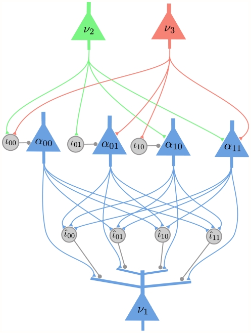
Implementation 4 is the neural implementation with auxiliary neurons and dendritic branches, that uses the factorized expansion of the log-odd ratio. As in Fig. 2 there is one auxiliary neuron for each possible value assignment to and . The connections from the neurons and (that carry the current values of the RVs and ) to the auxiliary neurons are the same as in Fig. 2, and when these RVs change their value, the auxiliary neuron that corresponds to the new value fires. Each auxiliary neuron connects to the principal neuron at a separate dendritic branch , and there is an inhibitory neuron connecting to the same branch. The rest of the auxiliary neurons connect to the inhibitory interneuron . The function of the inhibitory neuron is to shunt the active EPSP caused by a recent spike from the auxiliary neuron when the value of the and changes from to another value.

Figure 6. Implementation 5 for the Bayesian network shown in Fig. 1B .

Implementation 5 is the implementation with dendritic computation that is based on the factorized expansion of the log-odd ratio. RV occurs in two factors, and , and therefore receives synaptic inputs from and on separate groups of dendritic branches. Altogether the synaptic connections of this network of spiking neurons implement the graph structure of Fig. 1D.

Figure 7. Results of Computer Simulation II.

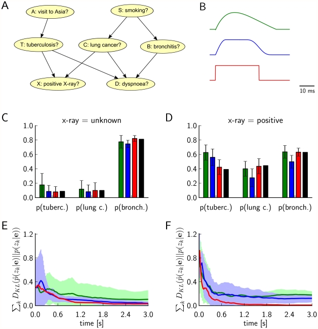
Probabilistic inference in the ASIA network with networks of spiking neurons that use different shapes of EPSPs. The simulated neural networks correspond to Implementation 2. The evidence is changed at from to (by clamping the x-ray test RV to 1). The probabilistic inference query is to estimate marginal posterior probabilities , , and . A) The ASIA Bayesian network. B) The three different shapes of EPSPs, an alpha shape (green curve), a smooth plateau shape (blue curve) and the optimal rectangular shape (red curve). C) and D) Estimated marginal probabilities for each of the diseases, calculated from the samples generated during the first 800 ms of the simulation with alpha shaped (green bars), plateau shaped (blue bars) and rectangular (red bars) EPSPs, compared with the corresponding correct marginal posterior probabilities (black bars), for in C) and in D). The results are averaged over 20 simulations with different random initial conditions. The error bars show the unbiased estimate of the standard deviation. E) and F) The sum of the Kullback-Leibler divergences between the correct and the estimated marginal posterior probability for each of the diseases using alpha shaped (green curve), plateau shaped (blue curve) and rectangular (red curve) EPSPs, for in E) and in F). The results are averaged over 20 simulation trials, and the light green and light blue areas show the unbiased estimate of the standard deviation for the green and blue curves respectively (the standard deviation for the red curve is not shown). The estimated marginal posteriors are calculated at each time point from the gathered samples from the beginning of the simulation (or from for the second inference query with ).

Figure 8. Spike raster of the spiking activity in one of the simulation trials described in Fig. 7 .

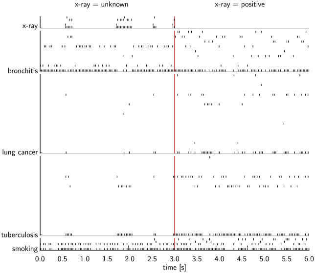
The spiking activity is from a simulation trial with the network of spiking neurons with alpha shaped EPSPs. The evidence was switched after 3 s (red vertical line) from to (by clamping the RV X to 1). In each block of rows the lowest spike train shows the activity of a principal neuron (see left hand side for the label of the associated RV), and the spike trains above show the firing activity of the associated auxiliary neurons. After the activity of the neurons for the x-ray test RV is not shown, since during this period the RV is clamped and the firing rate of its principal neuron is induced externally.

Figure 9. The randomly generated Bayesian network used in Computer Simulation III.

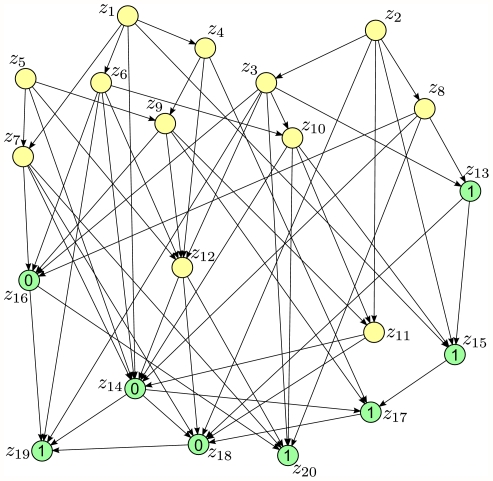
It contains 20 nodes. Each node has up to 8 parents. We consider the generic but more difficult instance for probabilistic inference where evidence is entered for nodes in the lower part of the directed graph. The conditional probability tables were also randomly generated for all RVs.

Figure 10. Results of Computer Simulation III.

Neural emulation of probabilistic inference through neural sampling in the fairly large and complex randomly chosen Bayesian network shown in Fig. 9. A) The sum of the Kullback-Leibler divergences between the correct and the estimated marginal posterior probability for each of the unobserved random variables , calculated from the generated samples (spikes) from the beginning of the simulation up to the current time indicated on the x-axis, for simulations with a neuron model with relative refractory period. Separate curves with different colors are shown for each of the 10 trials with different initial conditions (randomly chosen). The bold black curve corresponds to the simulation for which the spiking activity is shown in C) and D). B) As in A) but the mean over the 10 trials is shown, for simulations with a neuron model with relative refractory period (solid curve) and absolute refractory period (dashed curve.). The gray area around the solid curve shows the unbiased estimate of the standard deviation calculated over the 10 trials. C) and D) The spiking activity of the 12 principal neurons during the simulation from to , for one of the 10 simulations (neurons with relative refractory period). The neural network enters and remains in different network states (indicated by different colors), corresponding to different modes of the posterior probability distribution.

References

-
- Pearl J. Probabilistic Reasoning in Intelligent Systems. San Francisco, CA: Morgan- Kaufmann; 1988.
- Gold JI, Shadlen MN. The neural basis of decision making. Annu Rev Neuroscience. 2007;30:535–574. - PubMed
- Grimmett GR, Stirzaker DR. Probability and Random Processes. 3rd edition. Oxford University Press; 2001.
Publication types
MeSH terms
LinkOut - more resources
Full Text Sources
Other Literature Sources