. 2012:2012:937860.
doi: 10.1155/2012/937860. Epub 2011 Dec 21.

Free energy, value, and attractors

Affiliations

Free energy, value, and attractors

Karl Friston et al. Comput Math Methods Med. 2012.

Abstract

It has been suggested recently that action and perception can be understood as minimising the free energy of sensory samples. This ensures that agents sample the environment to maximise the evidence for their model of the world, such that exchanges with the environment are predictable and adaptive. However, the free energy account does not invoke reward or cost-functions from reinforcement-learning and optimal control theory. We therefore ask whether reward is necessary to explain adaptive behaviour. The free energy formulation uses ideas from statistical physics to explain action in terms of minimising sensory surprise. Conversely, reinforcement-learning has its roots in behaviourism and engineering and assumes that agents optimise a policy to maximise future reward. This paper tries to connect the two formulations and concludes that optimal policies correspond to empirical priors on the trajectories of hidden environmental states, which compel agents to seek out the (valuable) states they expect to encounter.


Figures

Figure 1
Figure 1
The free energy principle. The schematic shows the probabilistic dependencies (arrows) among the quantities that define free energy. These include the internal states of the brain μ˜(t) and quantities describing its exchange with the environment. These are the generalized sensory states s˜(t)=[s,s,s,]T and action a(t). The environment is described by equations of motion, which specify the trajectory of its hidden states and a mapping to sensory states. The quantities ϑ(x˜,θ) causing sensory states comprise hidden states and parameters. The hidden parameters control the equations (f, g) and precision (inverse variance) of random fluctuations (ω x(t), ω s(t)) on hidden and sensory states. Internal brain states and action minimize free energy (s˜,μ˜), which is a function of sensory states and a probabilistic representation q(ϑμ˜) of their causes. This representation is called the recognition density and is encoded by internal states that play the role of sufficient statistics. The free energy depends on two probability densities; the recognition density, q(ϑμ˜), and one that generates sensory samples and their causes, p(s˜,ϑm). The latter represents a probabilistic generative model (denoted by m), whose form is entailed by the agent. The lower panels provide alternative expressions for the free energy to show what its minimization entails. Action can only reduce free energy by increasing accuracy (i.e., selectively sampling sensory states that are predicted). Conversely, optimizing internal states makes the representation an approximate conditional density on the causes of sensory states. This enables action to avoid surprising sensory encounters. See main text for further details.
Figure 2
Figure 2
Self-organisation and the emergence of macroscopic behaviour. This figure shows a simple example of self-organisation using sixteen (Lorenz) oscillators that have been coupled to each other, so that each oscillator (with three microscopic states) sees the other oscillators. This is an example of a globally coupled map, where the dynamics of each oscillator conform to a classical Lorenz system. The equations of motion are provided in the left panel for each microstate, x j (i) : i ∈ 1,…, 16 : j ∈ 1,  2,  3, whose average constitutes a macrostate x j : j ∈ 1,  2,  3. Each oscillator has its own random fluctuations ω (i)(t) ∈ ℝ and speed exp⁡(ω i) ∈ ℝ+. The upper right panel shows the evolution of the microstates (dotted lines) and the macrostates (solid lines) over 512 time steps of one 1/32 second. The lower right panel, shows the first two macrostates plotted against each other to show the implicit attractor that emerges from self-organisation. The lower left panel shows the implicit synchronisation manifold by plotting the first states from successive pairs of oscillators (pink) and their averages (black) against each other. This simulation used low levels of noise on the motion of the microstates ω (i) ~ 𝒩(0, 22) and the log-rate constants ω i ~ 𝒩(0, 2−6) that disperse the speeds of each oscillator. The initial states were randomised by sampling from a Gaussian distribution with a standard deviation of eight.
Figure 3
Figure 3
The loss of macroscopic order and oscillator death. This figure uses the same format and setup as in the previous figure but here shows the loss of macroscopic order through incoherence (left) and oscillator death (right). Incoherence was induced by increasing the random fluctuations on the motion of states to ω (i) ~ 𝒩(0, 210). Oscillator death was induced by increasing the random dispersion of speeds along each oscillators orbit to ω i ~ 𝒩(0, 2−4), see [24]. The ensuing macroscopic states (lower panels) now no longer belong to the attracting set of the previous figure: 𝒜(ω) ⊂ 𝒪.
Figure 4
Figure 4
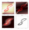
Value and cost functions of dynamical systems. This figure shows the value and cost functions of the Lorentz attractor used in the previous figures. These functions always exist for any global random attractor because value (negative surprise) is the log density of the eigensolution of the systems Fokker-Planck operator. This means, given any deterministic motion (flow) and the amplitude of random fluctuations (diffusion), we can compute the Fokker Planck operator Λ(f, Γ) and its eigensolution p = (Λ) and thereby define value V = ln⁡p. Having defined value, cost is just the expected rate of change of value, which is given by the deterministic flow and diffusion (see (23)). In this example, we computed the eigensolution or ergodic density using a discretisation of state-space into 96 bins over the ranges: [−32,  32]×[−32,  32]×[4,  64] and a diffusion tensor of Γ = (1/64) · I. The upper panels show the resulting value and (negative) cost functions for a slice through state-space at x 3 = 24. Note how cost takes large values when the trajectory (red line) passes through large value gradients. The lower left panel shows the resulting ergodic density as a maximum intensity projection over the third state. A segment of the trajectory producing this density is shown on the lower right.
Figure 5
Figure 5
The mountain car problem. The upper left panel shows the landscape or potential energy function φ(x, θ), with a minimum at position, x = −0.5 (green dot) that exerts forces on the car. The car is shown at the target position at the top of the hill at x = 1 (red dot). The equations of motion of the car are shown below. Crucially, at x = 0 the force is unity and cannot be overcome by the agent, because a squashing function −1 ≤ σ(a) ≤ 1 is applied to action. This means the agent can only access the target by starting on the left hill to gain enough moment to carry it up the other side. The right panels show the cost function and empirical priors (model of flow) that constitute the agent. Cost is a function of position and a hidden (e.g., physiological) state that plays a role of satiety c(x, z) = (16 · exp⁡(−64(x−1)2) − 1)·(tanh(8(z − 1)) − 1) − 1. When satiety is high, cost is uniformly negative; c(x, ) = −1. Conversely, when satiety is low cost becomes negative near, and only near, the target location; c(x, 0) = 1 − 32 · exp⁡(−64(x − 1)2). The equations of motion on the lower right are constructed to ensure that fixed points are only stable in regions of negative cost or divergence: see main text.
Figure 6
Figure 6
Examples of flow. This figure provides two examples of flow under two levels of action based on the equations of motion in the previous figure (the mountain car problem). These action-dependent flows provide a repertoire from which the agent has to compose a policy that conforms to its prior beliefs.
Figure 7
Figure 7
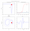
Active inference with generalised policies. This example shows how paradoxical but adaptive behaviour (moving away from a target to secure it later) emerges from simple priors on the motion of hidden states. These priors are encoded in a cost function c(x, 0) (upper left). The form of the agent's (generalised) policy ensures that divergence is positive or friction is negative in regions of positive cost, such that the car expects to go faster. The inferred hidden states (upper right: position in blue, velocity in green, and friction in red) show that the car explores its landscape until it encounters the target and friction increases dramatically to prevent it escaping (i.e., falling down the hill). The ensuing trajectory is shown in blue (lower left). The paler lines provide exemplar trajectories from other trials, with different starting positions. In the real world, friction is constant (one eighth). However, the car expects friction to change with position, enforcing exploration or exploitation. These expectations are fulfilled by action (lower right), which tries to minimise free energy.
Figure 8
Figure 8
Optimal itinerancy. This figure shows how itinerant dynamics can be constrained by a cost function, leading to a stable heteroclinic channel, in which unstable but attractive fixed points are visited in succession. Here, we have exploited the specification of cost in terms of satiety, which has been made a hidden (physiological) state. This makes cost time dependent and sensitive to the recent history of the agent's states. Placing dynamics on cost enables us to model sequential behaviour elicited by cost functions that are suppressed by the behaviour they elicit. The left panels show the true (upper) and modelled (lower) equations of motion on hidden states, where the latter are constrained by the cost function in Figure 5. Here, satiety increases with rewards (negative cost) and decays with first-order kinetics. The resulting behaviour is summarised in the right-hand side panels. The upper left panel shows the predictions of hidden states and prediction errors; where predictions are based upon the conditional beliefs about hidden states shown on the upper right. These predictions prescribe optimal action (lower right), which leads to the behavioural orbits shown on the lower left. The characteristic feature of the ensuing dynamics is a sequential return to unstable fixed points; denoted by the minimum of the potential landscape (green dots) and the cost-dependent (unstable) fixed point at the target location (red dots).

Similar articles

Cited by

References

    1. Friston K, Kilner J, Harrison L. A free energy principle for the brain. Journal of Physiology Paris. 2006;100(1–3):70–87. - PubMed
    1. Sutton RS, Barto AG. Toward a modern theory of adaptive networks: Expectation and prediction. Psychological Review. 1981;88(2):135–170. - PubMed
    1. Daw ND, Doya K. The computational neurobiology of learning and reward. Current Opinion in Neurobiology. 2006;16(2):199–204. - PubMed
    1. Dayan P, Daw ND. Decision theory, reinforcement learning, and the brain. Cognitive, Affective and Behavioral Neuroscience. 2008;8(4):429–453. - PubMed
    1. Niv Y, Schoenbaum G. Dialogues on prediction errors. Trends in Cognitive Sciences. 2008;12(7):265–272. - PubMed

Publication types

LinkOut - more resources