Virtual genomes in flux: an interplay of neutrality and adaptability explains genome expansion and streamlining

Abstract

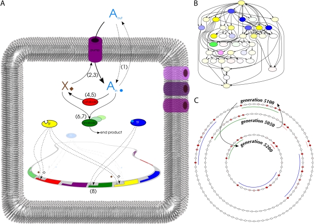
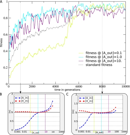
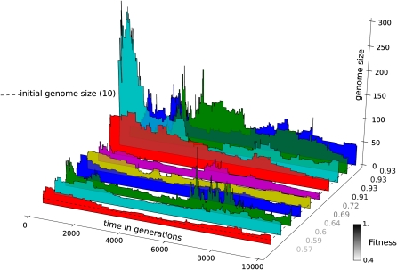
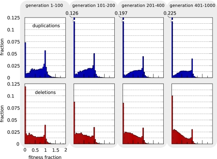
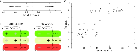
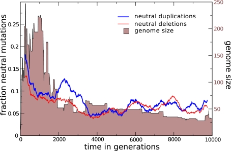
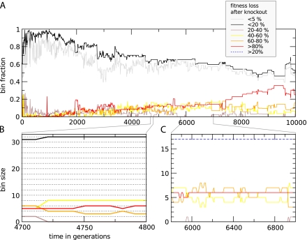
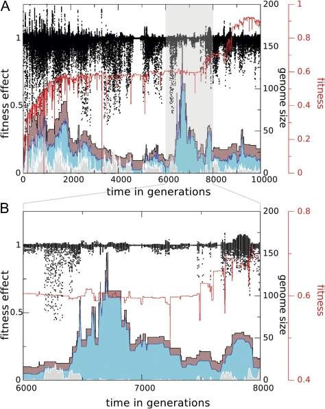
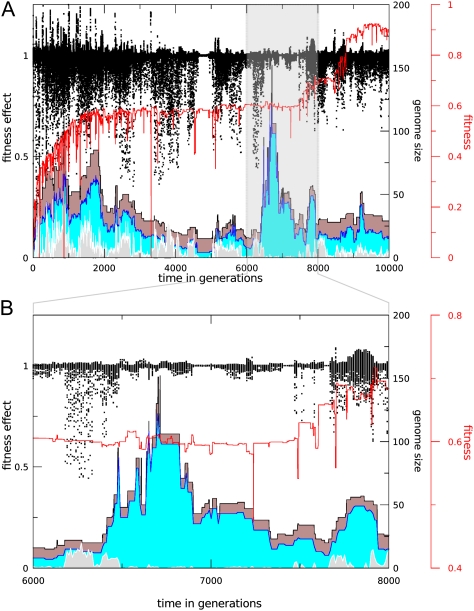
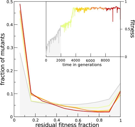
The picture that emerges from phylogenetic gene content reconstructions is that genomes evolve in a dynamic pattern of rapid expansion and gradual streamlining. Ancestral organisms have been estimated to possess remarkably rich gene complements, although gene loss is a driving force in subsequent lineage adaptation and diversification. Here, we study genome dynamics in a model of virtual cells evolving to maintain homeostasis. We observe a pattern of an initial rapid expansion of the genome and a prolonged phase of mutational load reduction. Generally, load reduction is achieved by the deletion of redundant genes, generating a streamlining pattern. Load reduction can also occur as a result of the generation of highly neutral genomic regions. These regions can expand and contract in a neutral fashion. Our study suggests that genome expansion and streamlining are generic patterns of evolving systems. We propose that the complex genotype to phenotype mapping in virtual cells as well as in their biological counterparts drives genome size dynamics, due to an emerging interplay between adaptation, neutrality, and evolvability.

FIG. 1.—

Schematic view and representations of the genome of virtual cells. (A) A permeates through the membrane (1) depending on relative concentrations inside and outside of the cell. Pumps consume X (2) to pump in A from the environment (3). Catabolic enzymes can convert A (4) into X (5) in a 1:4 ratio. Anabolic enzymes consume A (6) and X (7) to produce an unspecified end product. Protein expression (8) depends on the promoter strength and additional regulation of upstream TFs of the corresponding genes. The regulatory effect of a TF changes upon binding of its ligand (either A or X). (For reaction equations, see Materials and Methods). (B) GRN representation of a cell. Gene colors indicate the type as in (A), whereas color intensity indicates basal expression rate. (C) Circular genome representation of cells at three time points in evolution. Intensity of the red coloring of genes corresponds to fitness loss upon knockout of the gene. Colored arcs indicate syntenic regions that contain essential genes at different generation time points. Several genomic regions have been duplicated and deleted in the line of descent between the time points. The network in (B) corresponds with the middle circular genome at time = 5,050.

FIG. 2.—

Typical evolution of fitness in the line of descent of a run reaching a high fitness state. (A) Evolution of fitness in each standard environment separately (colored lines). The dotted black line is the standard fitness when the three environments are combined. (B and C) Snapshots of the regulatory response of the network for individuals at generations 1,000 (B) and 8,000 (C) in a log-log scale. Plotted are [A_in] and [X_in] as a function of [A_out]. For reference, the dashed vertical lines depict the [A_out] of the standard environments. The colors of reference lines correspond to those of the fitness lines in the upper graph. Genome size evolution of this run is depicted in figure 3, third graph from the back.

FIG. 3.—

An example of ten independent runs to illustrate the evolution of genome size. Plotted is the genome size in the line of descent. In the y-direction, the graphs of individual runs are ordered according to the fitness that the lineages have reached at the end of the run (fitness values in gray scale). The dashed line marks the average genome size of ten genes in the initial populations of all runs. There is a trend for the runs with larger initial genome expansions to be ordered toward the back.

FIG. 4.—

Large-scale duplication and deletion fitness landscapes. Mutant fitness data for 80 independent runs are created at 20 generation intervals during the first 1,000 generations of simulation. At these time points, 50 deletion and 50 duplication mutants are created for all 80 lineages and their fitnesses recorded in standard environments. Data of all runs are combined and lumped together into four time intervals (generations 1–100, 101–200, 201–400, and 401–1,000). Single duplication (deletion) events typically involve a stretch of adjacent genes of which we measure the net effect. The upper, blue histograms are duplications showing the fraction of mutants per fitness bin. Fitness values are the fractions of wild-type fitness that the mutants retain. For the lethal duplication mutants (fitnesses approaching 0), we annotate fractions separately in the last three time intervals. Lower, red histograms are deletions.

FIG. 5.—

Relationship between fitness, size, and the early fitness landscape. (A) The distribution of fitness values in 74 independent runs. (B) Biased fitness landscapes for future fit lineages. Runs were classified as fit if their final fitness exceeded 0.85. Fitness landscapes for mutants with duplications and deletions, respectively, were constructed for individuals in the line of descent during early evolution. At 20 generation intervals, 50 deletion and 50 duplication mutants of the lineages were created, and the fitness effects expressed as a fraction of the ancestral fitness. Fitness landscapes of fit and unfit lineages were combined and the time points lumped into two time intervals: generations 1–100 and 101–200, respectively. Plus and minus signs denote over- and underrepresentation of a class of fitness effects in a given time interval for the fit set, as measured with Mann–Whitney U tests. Dark signs are significant (P < 0.05) and grayed signs denote a bias under a lower threshold (P < 0.1), whereas equal signs denote no bias. (C) (early) genome size affects late fitness. In 40 runs with a fixed genome size (see main text for details), the late fitness is plotted as a function of the genome size.

FIG. 6.—

Fractions of neutral duplications and deletions in random mutation essays. The fraction of mutants with either duplication or deletion mutations that show no fitness effect is plotted over evolutionary time in the line of descent at ten generation intervals, as a 50 point running average. For reference, the genome size is plotted in the background.

FIG. 7.—

Specialization of genes in the GRN. Genes have been assigned to bins according to the fitness loss of the cell after knockout of the gene. Five main bins exist for all 20% fitness partitions. The <5%-bin (gray line) is a subset of the <20%-bin (black line). (A) shows fractions that the respective bins take up in the whole network. (B and C) show the actual bin sizes in numbers of genes. In (B), between generation 4,700 and 4,725, we see that one gene moves to the <20%-bin (black) from the 20%- to 40%-bin (brown), whereas a second gene from the brown bin increases its contribution, moving into the 40%- to 60%-bin (yellow). At the same time, two genes from the 60%- to 80%-bin (orange) also move down to the yellow bin. In (C), the >20%-bin (blue dashed line) sums over all main bins that have a higher than 20% fitness loss. This remains constant, whereas the contributions of individual genes are continuously changing.

FIG. 8.—

Evolution of the mutational load associated with neutral genes. (A) Individual mutant fitness fractions (black dots), illustrating the breadth of mutational effects, and a simple mutational load measure (gray graph) are shown together with the total genome size (brown graph) and the set of neutral genes (cyan). (B) The corresponding evolution of the fitness of the ancestor (red) and that of the population as a whole (orange, averaged).

FIG. 9.—

Neutral genome fluctuations. As in figure 8, A shows mutational load of neutral genes (black dots), total genome size (brown), the subset of neutral genes (cyan), and the mutational load measure (gray), but this time overlayed with fitness in the line of descent (red). In the highlighted area (seen in more detail in B), fitness remains initially constant, whereas the neutral gene complement increases drastically. The most significant size increases occur after the mutational load has gone down a very low level. Subsequently, when the genome has shrunk but is still at a significantly higher level than before the sudden increase, fitness starts to go up, eventually reaching the high fitness regime after a 1,500 generation phase of adaptive evolution. It appears that the new adaptive phase is triggered by the initially neutral genome size fluctuations.

FIG. 10.—

Long-term fitness landscape evolution. A set of averaged fitness landscapes of 2,000 generation intervals in the line of descent of a single run is plotted. Fitness landscapes are constructed by inducing rounds of mutations in individuals in the lineage at ten generation intervals. The mutation scheme is identical to that used in standard evolutionary runs, except that a 5-fold higher mutation rate is used, resulting in a 0.5 chance for all mutational operators to affect an individual gene. Colors of graphs correspond to the colored section in the inset, showing the evolution of fitness.

References

1. Aldana M, Balleza E, Kauffman S, Resendiz O. Robustness and evolvability in genetic regulatory networks. J Theor Biol. 2007;245:433–448. - PubMed
1. Ames RM, et al. Gene duplication and environmental adaptation within yeast populations. Genome Biol Evol. 2010;2:591–601. - PMC - PubMed
1. Andersson DI, Hughes D. Gene amplification and adaptive evolution in bacteria. Annu Rev Genet. 2009;43(1):167–195. - PubMed
1. Archibald JD. Divergence times of eutherian mammals. Science. 1999;285(5436):2031.
1. Battistuzzi F, Feijao A, Hedges SB. A genomic timescale of prokaryote evolution: insights into the origin of methanogenesis, phototrophy, and the colonization of land. BMC Evol Biol. 2004;4(1):44. - PMC - PubMed
Publication types