Cross-frequency phase-phase coupling between θ and γ oscillations in the hippocampus

Abstract

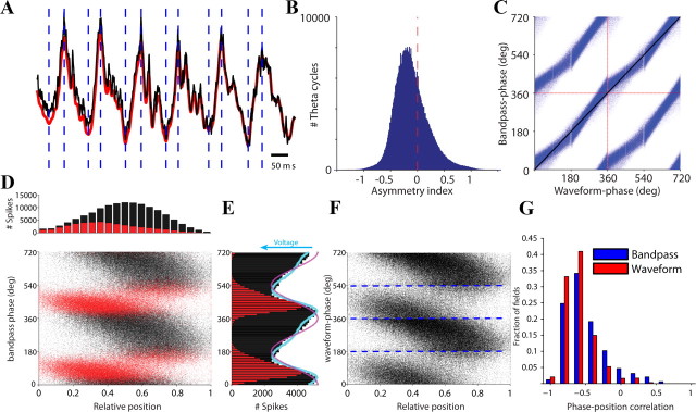
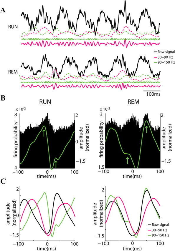
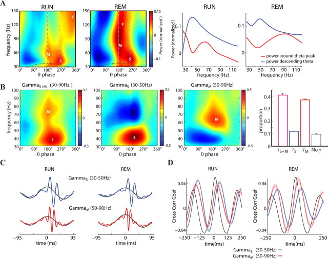
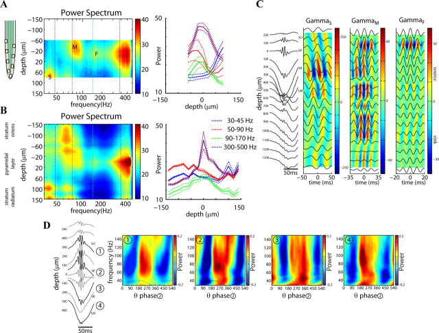
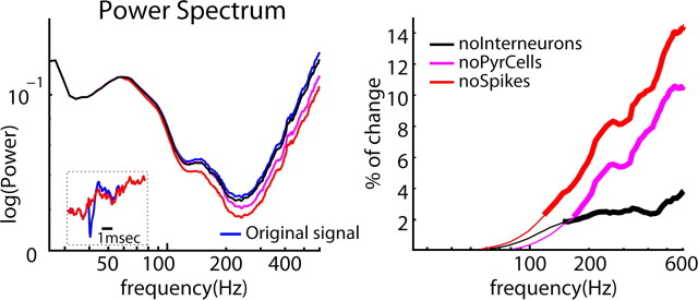
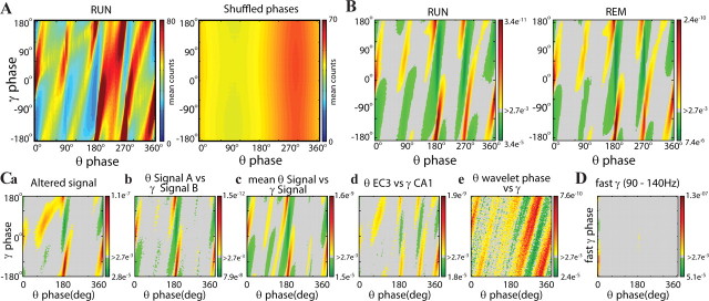
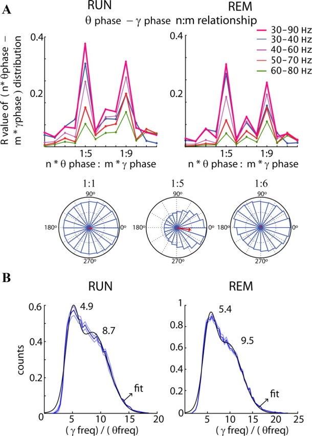
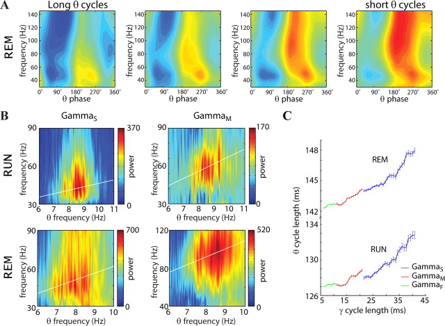
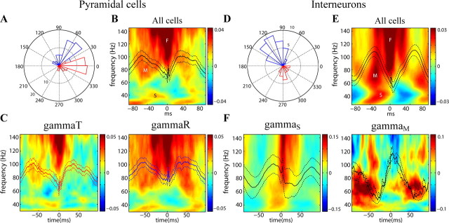
Neuronal oscillations allow for temporal segmentation of neuronal spikes. Interdependent oscillators can integrate multiple layers of information. We examined phase-phase coupling of theta and gamma oscillators in the CA1 region of rat hippocampus during maze exploration and rapid eye movement sleep. Hippocampal theta waves were asymmetric, and estimation of the spatial position of the animal was improved by identifying the waveform-based phase of spiking, compared to traditional methods used for phase estimation. Using the waveform-based theta phase, three distinct gamma bands were identified: slow gamma(S) (gamma(S); 30-50 Hz), midfrequency gamma(M) (gamma(M); 50-90 Hz), and fast gamma(F) (gamma(F); 90-150 Hz or epsilon band). The amplitude of each sub-band was modulated by the theta phase. In addition, we found reliable phase-phase coupling between theta and both gamma(S) and gamma(M) but not gamma(F) oscillators. We suggest that cross-frequency phase coupling can support multiple time-scale control of neuronal spikes within and across structures.

Figure 1.

Theta waves are asymmetric. A, Example trace of LFP from the CA1 pyramidal cell layer during a RUN. The black line shows the unfiltered LFP (1–1000 Hz; median of all CA1 recording sites); red trace is the bandpass-filtered (1–80 Hz) derivative. Vertical dashed lines mark local minima and maxima that were used subsequently to align individual theta cycles. B, Distribution of the asymmetry index: ratio of the duration of the ascending and descending parts expressed on a logarithmic scale. Zero corresponds to a symmetric theta waveshape. C, Comparison of bandpass-filtered (4–12 Hz) and waveform-based spike phases (blue dots). Two oscillation cycles (separated by dashed red lines) are shown for clarity. Identical phase estimates lie on the diagonal black line. Vertical stripes are due to discretization and sampling rate. D, Spike phase precession in a single rat. Bottom, For each spike, theta phase was determined from the filtered (4–12 Hz) LFP, and spike phases are plotted against the position of the animal within the field. Red and black dots denote spikes on the ascending and descending parts of the theta cycle, respectively. Top, Number of spikes at a given relative position of the rat in the place field. E, Spike density at different theta phases. For spikes with the same theta phase, the median of the simultaneously recorded voltage values in the raw LFP was determined. The resulting values were scaled to the peak and trough of the spike phase histogram (blue line). The polarity of the blue line is switched to match the histograms. A cosine wave (red line) is also shown to illustrate phase relationships. F, Spike phase precession for the same rat shown in D. The phases of the spikes were computed from the waveform-based theta phase. Blue lines represent detected peaks and troughs. G, Distribution of spike phase-position correlations (3 rats) calculated for waveform-based phases and bandpass (4–12 Hz) phases.

Figure 2.

State dependence of theta phase locking of gamma frequencies. A, Example raw trace (black; 1–1250 Hz) from the CA1 pyramidal cell layer during RUN (top) and REM (bottom). The solid magenta (30 to 90 Hz) and green (90 to 150 Hz) lines show filtered LFP and the respective dashed lines the (z-scored) power for each band. B, Probability of pyramidal cell firing (n = 372) related to the reference theta wave troughs (time 0). The superimposed green line shows the temporal distribution of mean LFP power in the 90 to 150 Hz band (z-score values). Note units have two maxima during the theta cycle, largely corresponding to the two peaks of the 90–150 Hz power (arrows). C, Temporal relationship between theta trough-triggered raw LFP (black) and integrated power in the 30 to 90 Hz band (magenta). The amplitude values of the signals are z-scored. Note similar theta phase relationship with 30 to 90 Hz power and different preferred theta phases of 90 to 150 Hz power during RUN and REM.

Figure 3.

Discrete low (S), middle (M), and fast (F) bands of gamma oscillations. A, Left panels show the mean wavelet power between 30 and 150 Hz as a function of the waveform-based theta cycle phases (bin, 9°) for RUN and REM (0°, trough of theta cycle). Right panels show the mean power around the peak (red line, mean between 125 and 216°) and during the descending part (blue line, mean between 216 and 288°) of the theta wave. The dashed vertical lines in the left panels represent the centers of the windows used for the calculation of the mean power. Note different theta phase preference of gamma_M (50–90 Hz, near theta peak) and gamma_S (30–50 Hz, on the descending phase of theta). Note also phase shifting of gamma_F (90–150 Hz; ε band) from the trough of theta during RUN to the peak of theta during REM (as in Fig. 2). Power values were normalized by frequency band by its mean and SD for each session. Blue and red colors emphasize relative power distributions. B, Example average wavelet maps of theta cycles during RUN with both gamma_S and gamma_M, gamma_S only, and gamma_M only. Right, Population distribution of theta cycles (mean ± SE) with both gamma_S and gamma_M, gamma_S only, gamma_M, and cycles with no detected gamma. The threshold for the inclusion was >2 SD of gamma power (relative to the session mean) in a given theta cycle. S, M, and F mark gamma_S, gamma_M and gamma_F (ε) bands, respectively. C, Gamma trough-triggered LFP. Troughs of filtered (30–50 Hz, blue; 50–90 Hz, magenta) traces >2 SD of the session mean were detected and used to trigger LFP (1–1250 Hz, colored lines) or theta-filtered LFP (4–12 Hz; black lines) during RUN and REM sessions. Traces are aligned to the peak of the theta LFP. D, Cross-correlation between theta LFP (4–12 Hz) and power of filtered (gamma_S, 30–50 Hz; gamma_M, 50–90 Hz) gamma waves (mean ± SE). Black line, Autocorrelation of the theta band.

Figure 4.

Distribution of gamma bands within the CA1 pyramidal layer. A, Color-coded power spectra from each of the eight vertical recording sites by the silicon probe, smoothed across depth. Data are from a single session. Right, Depth distribution of the mean (±SE) power in different frequency bands, the means of which correspond to the dotted lines in the left panel. Note the different depth distribution of gamma_S (S), gamma_M (M) and gamma_F (F, ε) bands. B, Average of nine recording sessions from three rats (2 sessions were excluded due to the presence of 60 Hz noise; inclusion of those 2 sessions does not change the result). The channel with the highest power in the >200 Hz band was used to align the traces from the different recordings sites. C, Left, average wideband LFPs at different depths, triggered by the trough of filtered ripples. Depth 0 (reference) is the middle of the pyramidal cell layer. Right, Average filtered LFPs in the gamma_S, gamma_M, and gamma_F during RUN episode triggered by gamma peak. Color plots are the derived current source density map for the three gamma bands. Only epochs with a peak power above >2 SD of the session mean were included. Note different time scales, different source/sink strengths, and distinct depth profiles for the three gamma bands. D, Theta phase-related distribution of wavelet power at different depths (1–4) in a RUN session. Note that while gamma_S is most prominent in the middle of stratum radiatum (Site 3), the power of gamma_M is largest in stratum oriens/pyramidale and lacunosum-moleculare (Sites 1, 2 and 4). The wavelet power plots are shown for one and a half cycles of theta (from 0 to 540°). SO, Stratum oriens; SP, stratum pyramidale; SR, stratum radiatum; LM, stratum lacunosum moleculare.

Figure 5.

Spike contribution to gamma_F. Left, Mean power of the original “whitened” signal from the CA1 pyramidal layer (blue) and its despiked derivatives. Magenta, Pyramidal cells spikes removed; black, interneurons removed; red, spikes of both cell classes removed. Inset, Single spike of an example pyramidal cell (blue) and its surrogate (red) after removal the mean spike from the LFP. Right, Percentage of change of power (1 − despike power/original power) at different frequencies after despiking the LFP. Thick lines indicate significantly different values between the original and despiked LFPs (p < 0.01, t test). noInterneurons, After removal of spikes of putative interneurons; noPyrCells, after removal of spikes of pyramidal cells; noSpikes, after removal of all spikes.

Figure 6.

Phase–phase coupling between theta and gamma_S and gamma_M oscillations. A, Phase–phase plots for original (2D histograms, averaged across n = 11 sessions in 3 rats) and shuffled signals (right) during RUN sessions. B, Plots of significant theta phase–gamma phase pixels for RUN and REM periods. Gray corresponds to p values of >0.027, considered here as nonsignificant. Values with less or more than the expected values (p < 0.027) are colored green and red/yellow, respectively. Ca, Theta phases from an altered signal versus gamma phases from the original signal. Cb, Theta phases from the signal recorded at Site A versus gamma phases from the signal recorded at Site B (>600 μm) in the pyramidal layer. Cc, Gamma phases from the signal at Site A versus theta phases from the mean signal from all other electrodes. Cd, Theta phases from entorhinal cortex Layer 3 versus gamma phases from CA1 pyramidal cell layer. Ce, Wavelet theta phases versus gamma phases. Note the reliable relationship between theta and gamma phases in all comparisons. D, Fast gamma phases (epsilon; 90 to 150 Hz) versus theta phases. C and D correspond to RUN episodes.

Figure 7.

Phase–phase (n:m) coupling between theta and gamma oscillations. A, Top, Mean radial distance values (R values) from the distribution of the difference between theta and gamma phases calculated for different n:m relationships during RUN and REM. The procedure was repeated for several filtered bands in the gamma frequency band. Note large peaks at 5 (mainly for band 30–40 Hz) and 9 (mainly for 50–80 Hz). The bottom panels show examples of the distribution of the difference between theta and gamma phases for three different n:m relationships (1:1, 1:5, and 1:6). Only the distribution using the 1:5 ratio shows a unimodal distribution around 0 with a high R value. B, Distribution of the ratios between gamma (30–90 Hz) and theta frequency (4–12 Hz; blue lines, mean ± SE). For every theta cycle, the maximum in the power spectrum in the range between 30 and 90 Hz was compared with the corresponding theta cycle frequency (1/duration). The black line is the fitted Gaussian to the distribution with the center of mass for each function displayed (with a confidence of 95%). Note the peaks at ∼5 (gamma_S) and ∼9 (gamma_M).

Figure 8.

Correlation between theta and gamma frequencies. A, Mean wavelet power between 30 and 150 Hz versus theta phases divided according to theta cycle length from long (or slow; 5.5 Hz; left) to short (or fast; 8.1 Hz; right). B, For each theta wave, the mean power around the peak (between 125 and 216°) and on the descending phase (between 216 and 288°) was calculated and sorted by theta cycle length. During RUN, the line fitted to the power around the peak versus theta frequency has a slope of 7.15 (gamma_M, R² = 0.67; p < 0.01) and a slope of 3.5 for the power in descending phase (gamma_S, R² = 0.41; p < 0.01). During REM, the slopes are 9.22 (gamma_M, R² = 0.62; p < 0.01) and 4.28 (gamma_S, R² = 0.65; p < 0.01), respectively. C, Theta cycle length as a function of gamma cycle length (mean ± SE). Gamma cycle length was measured as the distance between peaks only for pairs with a power >2 SD of the session mean. Note that theta and gamma_S and gamma_M frequencies covary during both RUN and REM, but with different ratios.

Figure 9.

Unit correlations of gamma oscillations. A, Polar plot showing the preferred gamma phases of pyramidal cells referenced to gamma oscillation in CA1 pyramidal layer. Two groups are separated on the bases of gamma phase preference in the 30–90 Hz band (Senior et al., 2008). Neurons near the trough (0–30° or 240–360°; red) are referred to as gammaT neurons and neurons on the rising phase of the gamma wave (30–240°; blue) as gammaR neurons. B, Spike-sampled wavelet map during RUN for all pyramidal cells significantly modulated by gamma (n = 109). Spike-sampled maps were constructed by averaging wavelet power surrounding every spike. S, M, and F mark gamma_S, gamma_M and gamma_F (ε) bands, respectively. C, Spike-sampled wavelet maps shown separately for gammaT (n = 52) and gammaR (n = 57) pyramidal cells. D, Polar plot with the preferred gamma phases of putative interneurons. Note the bimodal phase distribution. E, Spike-sampled wavelet map during RUN for interneurons (n = 53). F, Spike-sampled wavelet maps for interneurons significantly phase-locked to gamma_S (n = 9) or gamma_M (n = 2) oscillations only. Spike-triggered LFPs (mean ± SE) are superimposed on the wavelet maps.

References

1. Bragin A, Jandó G, Nádasdy Z, Hetke J, Wise K, Buzsáki G. Gamma (40–100 Hz) oscillation in the hippocampus of the behaving rat. J Neurosci. 1995;15:47–60. - PMC - PubMed
1. Bressler SL, Freeman WJ. Frequency analysis of olfactory system EEG in cat, rabbit, and rat. Electroencephalogr Clin Neurophysiol. 1980;50:19–24. - PubMed
1. Buhl DL, Harris KD, Hormuzdi SG, Monyer H, Buzsáki G. Selective impairment of hippocampal gamma oscillations in connexin-36 knock-out mouse in vivo. J Neurosci. 2003;23:1013–1018. - PMC - PubMed
1. Burns SP, Xing D, Shapley RM. Is gamma-band activity in the local field potential of v1 cortex a “clock” or filtered noise? J Neurosci. 2011;31:9658–9664. - PMC - PubMed
1. Buzsáki G. Rhythms of the brain. New York: Oxford UP; 2006.
Publication types
LinkOut - more resources