Adaptation of binaural processing in the adult brainstem induced by ambient noise

Abstract

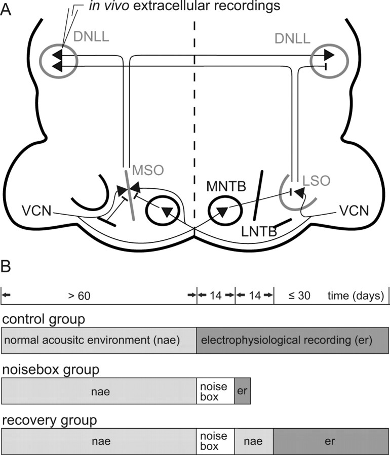
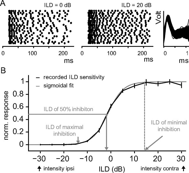
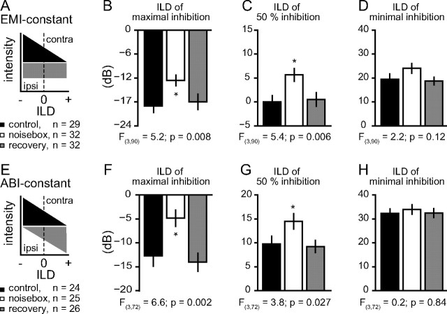
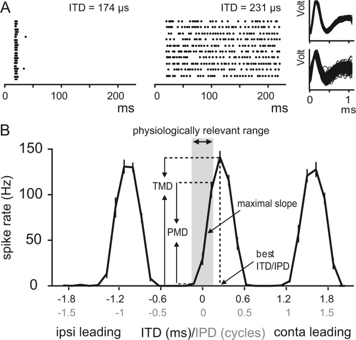
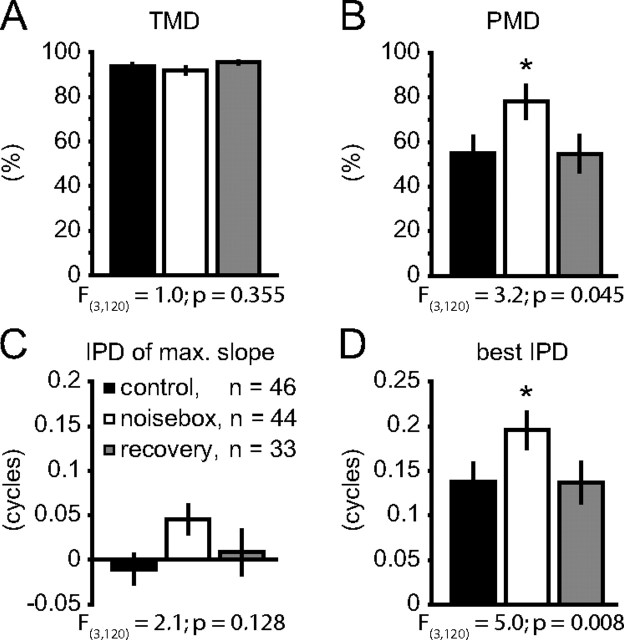
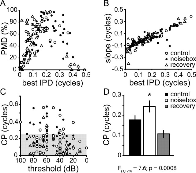
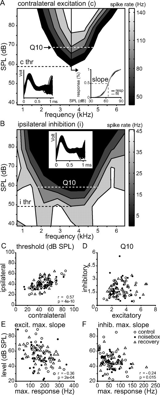
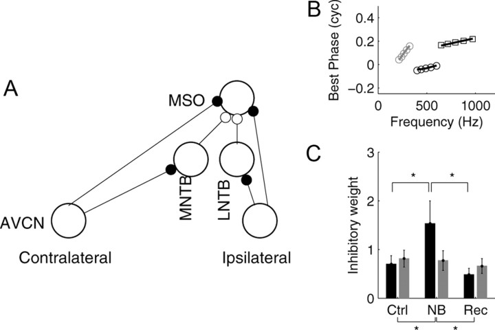
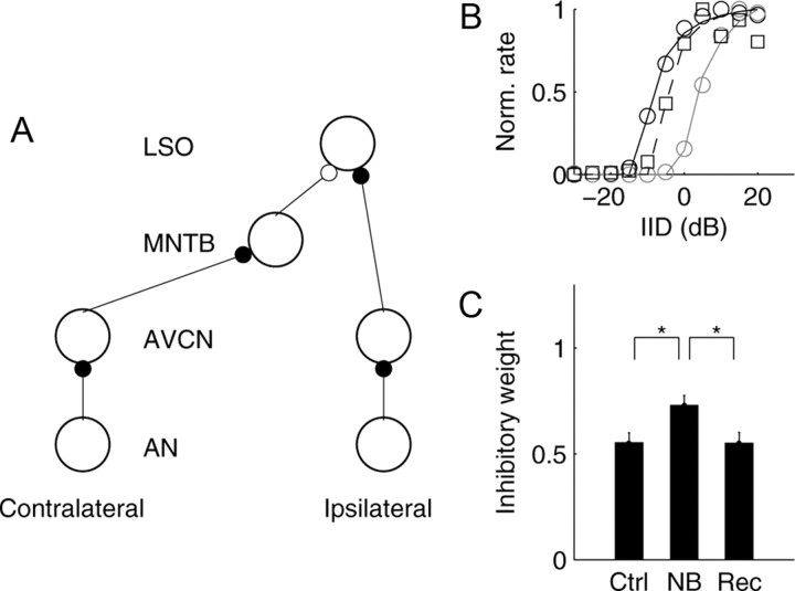
Interaural differences in stimulus intensity and timing are major cues for sound localization. In mammals, these cues are first processed in the lateral and medial superior olive by interaction of excitatory and inhibitory synaptic inputs from ipsi- and contralateral cochlear nucleus neurons. To preserve sound localization acuity following changes in the acoustic environment, the processing of these binaural cues needs neuronal adaptation. Recent studies have shown that binaural sensitivity adapts to stimulation history within milliseconds, but the actual extent of binaural adaptation is unknown. In the current study, we investigated long-term effects on binaural sensitivity using extracellular in vivo recordings from single neurons in the dorsal nucleus of the lateral lemniscus that inherit their binaural properties directly from the lateral and medial superior olives. In contrast to most previous studies, we used a noninvasive approach to influence this processing. Adult gerbils were exposed for 2 weeks to moderate noise with no stable binaural cue. We found monaural response properties to be unaffected by this measure. However, neuronal sensitivity to binaural cues was reversibly altered for a few days. Computational models of sensitivity to interaural time and level differences suggest that upregulation of inhibition in the superior olivary complex can explain the electrophysiological data.

Figure 1.

Experimental conditions. A, Schematic drawing of the first stages of the binaural auditory pathway, including the SOC and the DNLL where the in vivo extracellular recordings were made. Inputs and outputs of the MSO are illustrated for the left hemisphere, whereas inputs and outputs of the LSO are shown in the right hemisphere. Triangles indicate excitatory inputs. Bars indicate inhibitory inputs. VCN indicates ventral cochlear nucleus. B, Schematic diagram of the experimental design. The light gray boxes indicate how long the animals spent in a normal acoustic environment (nae), the white boxes indicate the times spent in the noisebox. The dark gray boxes mark the periods during which electrophysiological recordings (er) were made.

Figure 2.

Example of the response characteristics of an ILD-sensitive neuron in the DNLL. A, Raster plots show sustained responses (cell_230207_05; BF = 2500 Hz) to a 200 ms pure-tone stimulus at BF presented with ILDs of 0 and 20 dB. The shapes of the APs are displayed on the right. B, ILD function of the neuron shown in A. Negative ILDs indicate that the ipsilateral stimulus is louder than the contralateral stimulus. The parameters used to characterize the ILD sensitivity of the neurons are illustrated in gray.

Figure 3.

Effects of noise exposure on ILD sensitivity. A, E, Schematics depicting the two methods used to construct ILD stimuli: keeping EMI (20 dB above threshold) or ABI (20 dB above threshold) constant. B–D, F–H, Population averages of the ILD of maximal inhibition (B, F), ILD of 50% inhibition (C, G), and the ILD of minimal inhibition (D, H) are shown for the three study groups. Data in B–D correspond to EMI stimuli. Data in F–H correspond to ABI stimuli. Error bars indicate SEM. The asterisks indicate that the values for the noisebox group differ significantly (p < 0.05, ANOVA) from those for the control and recovery groups.

Figure 4.

Example of the response characteristics of an ITD-sensitive neuron in the DNLL. A, Raster plots of an onset neuron (left, cell_1504_02; BF = 600 Hz) and a sustained neuron (middle, cell_0704_05; BF = 600 Hz) to a 200 ms pure-tone stimulus at the neuron's BF and best ITD. The AP waveforms of the onset (top) and the sustained (bottom) neurons are displayed on the right. B, Example of an ITD (IPD, gray axis labels) function. The neuronal response rate (sustained neuron in A) is plotted against the ITD (black) and IPD (gray) of the stimulus. The gray area indicates the physiologically relevant range of ITDs for a gerbil (±135 μs). ITD sensitivity is characterized by four parameters: total modulation depth (TMD), physiological modulation depth (PMD), IPD at maximal slope, and best IPD.

Figure 5.

Effects of noise exposure on ITD sensitivity. A, Population averages of total modulation depth (TMD). B, Population averages of physiological modulation depth (PMD). C, IPD at maximal slope. D, Best IPD. Error bars indicate SEM. The asterisks indicate that the values for the noisebox group differ significantly (p < 0.05, ANOVA) from those for the control and recovery groups.

Figure 6.

Correlations between parameters used to characterize ITD sensitivity. A, Physiological modulation depth (PMD) and best IPD. B, IPD at maximal slope and best IPD. C, CP and neuronal threshold. Each ITD-sensitive DNLL neuron is represented by a symbol (squares, control; circles, noisebox; triangles, recovery). D, Population average of the CPs. The asterisks indicate that the values for the noisebox group differ significantly (p < 0.05, ANOVA) from those for the control and recovery groups.

Figure 7.

Effects of noise exposure on monaural response properties of high CF neurons. A, B, Response areas for contralateral excitatory (A) and ipsilateral inhibitory (B) inputs to a single DNLL cell (cell_060803_02; in both cases CF = 3.6 kHz). In A, regions with only spontaneous or subthreshold activity are also depicted in white. A, The inhibitory inputs were measured by binaural stimulation, setting the contralateral excitatory input to 20 dB above threshold at CF. The excitatory threshold [contralateral (c)] was defined as the lowest intensity that evoked 20% of the maximal response (c thr = 59 dB SPL; Q₁₀ = 1.6). B, The inhibitory threshold [ipsilateral (i)] was defined as the lowest intensity that inhibited 40% of the response to contralateral stimulation (i thr = 49 dB SPL; Q₁₀ = 1.1). C–F, Correlations between the analyzed parameters for each cell: inhibitory versus excitatory threshold (C), inhibitory Q₁₀ versus excitatory Q₁₀ (D), and maximal responses versus level at the maximum slope of the excitatory (E) and the inhibitory (F) rate-level function.

Figure 8.

Model of ILD sensitivity in the LSO. A, Circuit diagram. Each large circle is modeled by a nonlinear input–output function (Reed and Blum, 1999). Black disks indicate excitatory synapses (weight 1). The white disk indicates the inhibitory synapse from MNTB to LSO. AN indicates auditory nerve. B, Three examples of ILD response functions from the model (lines) and data points (symbols) to which the model is fitted. C, Mean inhibitory weights calculated from fits to response functions for the three groups of animals. Error bars indicate SEM. *p < 0.05 for an unpaired t test.

Figure 9.

Model of ITD sensitivity in the MSO. A, Circuit diagram. Black disks indicate excitatory synapses. White disks indicate inhibitory synapses. Model responses are fitted to phase–frequency curves, i.e., best IPD as a function of stimulus frequency. B, Three examples of phase–frequency curves. Model results are depicted as solid lines. Best IPDs derived from the data are depicted as symbols. C, Mean inhibitory weights (black, ipsilateral; gray, contralateral) from fits to the phase–frequency curves of the three groups of animals. Error bars indicate SEM. *p < 0.05 for an unpaired t test. The asterisks below the graphs indicate significance of the sum of ipsi- and contralateral weights).

References

-
- Alvarado JC, Fuentes-Santamaria V, Henkel CK, Brunso-Bechtold JK. Alterations in calretinin immunostaining in the ferret superior olivary complex after cochlear ablation. J Comp Neurol. 2004;470:63–79. - PubMed
- Batra R, Kuwada S, Fitzpatrick DC. Sensitivity to interaural temporal disparities of low- and high-frequency neurons in the superior olivary complex. I. Heterogeneity of responses. J Neurophysiol. 1997;78:1222–1236. - PubMed
- Blauert J. Spatial hearing: the psychophysics of human sound localization. Cambridge, MA: MIT; 1997.
Publication types
MeSH terms
LinkOut - more resources
Full Text Sources