Estimating abundances of retroviral insertion sites from DNA fragment length data

Abstract

Motivation: The relative abundance of retroviral insertions in a host genome is important in understanding the persistence and pathogenesis of both natural retroviral infections and retroviral gene therapy vectors. It could be estimated from a sample of cells if only the host genomic sites of retroviral insertions could be directly counted. When host genomic DNA is randomly broken via sonication and then amplified, amplicons of varying lengths are produced. The number of unique lengths of amplicons of an insertion site tends to increase according to its abundance, providing a basis for estimating relative abundance. However, as abundance increases amplicons of the same length arise by chance leading to a non-linear relation between the number of unique lengths and relative abundance. The difficulty in calibrating this relation is compounded by sample-specific variations in the relative frequencies of clones of each length.

Results: A likelihood function is proposed for the discrete lengths observed in each of a collection of insertion sites and is maximized with a hybrid expectation-maximization algorithm. Patient data illustrate the method and simulations show that relative abundance can be estimated with little bias, but that variation in highly abundant sites can be large. In replicated patient samples, variation exceeds what the model implies-requiring adjustment as in Efron (2004) or using jackknife standard errors. Consequently, it is advantageous to collect replicate samples to strengthen inferences about relative abundance.

Fig. 1.

versus Length. Estimates are provided for the replicates of sample I1 (solid lines) and sample B2 (dashed lines). The insert (dotted box) shows the corresponding calibration curves and an empirical calibration curve (thick line—see text).

Fig. 2.

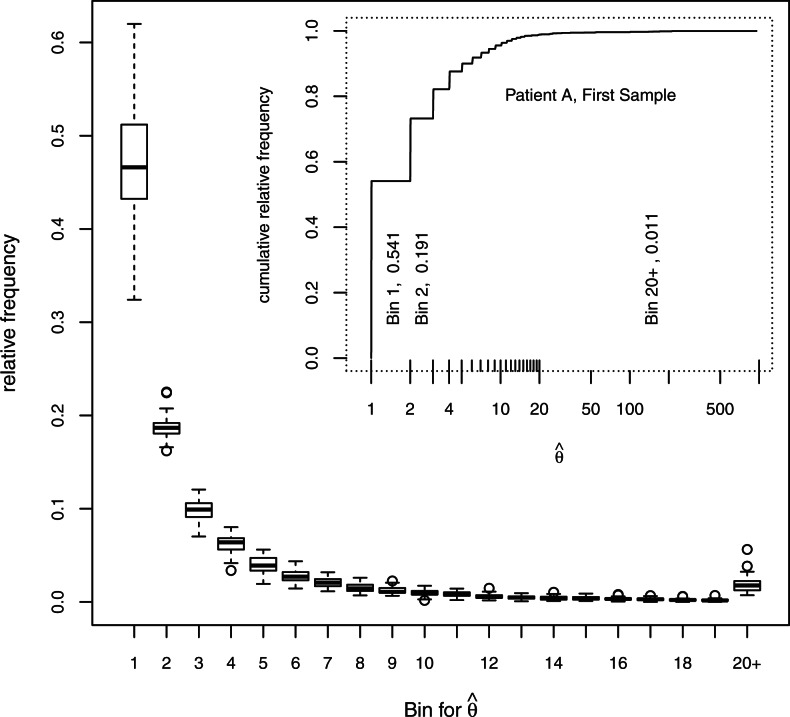
Abundances of integration sites. The insert shows the cumulative frequency distribution for one sample, the bins used for relative frequencies in the larger plot enclosed by tick marks above the x-axis and the relative frequencies for three of the bins. Boxplots show the relative frequencies of each bin of for 33 samples. The box covers the first through third quartiles of the data, the central line of each box shows the median, the whiskers extend to the closer of the extreme or to 1.5 times the height of the box away from the box, and circles show points, if any, that lie beyond the whiskers.

Fig. 3.

Relative abundance of integration sites. A boxplot for the relative abundances of each sample is shown. The width of each box and its whiskers is quite narrow compared with the range of the data, and every sample has sites (seen as dots) that lie well beyond the box and whisker. The samples are in chronological order in each panel—lower is earlier.

Fig. 4.

Change statistics distribution. The Normal density (A) and the empirical distribution of change statistics (D) are used to form the Normal probability qq–plot (C). Linearity of the qq-plot is used to visually assess goodness-of-fit to the theoretical density. The plot would follow the line of identity in (C), if the data were Normal with unit variance. The linearity of the central portion is expected when there is a mixture of null and non-null hypotheses, but an adjustment is needed to match the null variance. (B) The cutoffs for a 20% FDR after accounting for the apparent null variance.

Fig. 5.

Changes in abundance. The relative abundances are plotted against sample date. The vertical axis uses a cube root scale for better visualization. Gray lines join the values between first and second samples and between the second and third samples.Black lines overlay adjacent pairs with abundances different at FDR <0.20. Dashed lines overlie both pairs when first and third samples differ at FDR<0.20.

References

-
- Baker S. The multinomial-poisson transformation. Statistician. 1994;43:495–504.
- Chao A. Estimating the population size for capture-recapture data with unequal catchability. Biometrics. 1987;43:783–791. - PubMed
Publication types
MeSH terms
Grants and funding
LinkOut - more resources
Full Text Sources
Other Literature Sources