Importance of factors determining the effective lifetime of a mass, long-lasting, insecticidal net distribution: a sensitivity analysis

Abstract

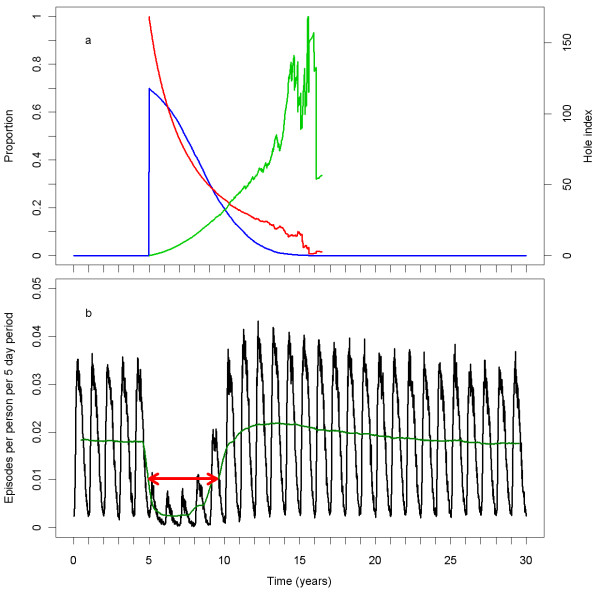
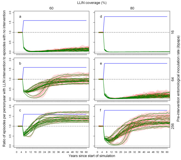
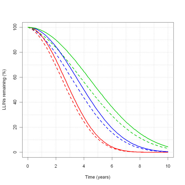
Background: Long-lasting insecticidal nets (LLINs) reduce malaria transmission by protecting individuals from infectious bites, and by reducing mosquito survival. In recent years, millions of LLINs have been distributed across sub-Saharan Africa (SSA). Over time, LLINs decay physically and chemically and are destroyed, making repeated interventions necessary to prevent a resurgence of malaria. Because its effects on transmission are important (more so than the effects of individual protection), estimates of the lifetime of mass distribution rounds should be based on the effective length of epidemiological protection.

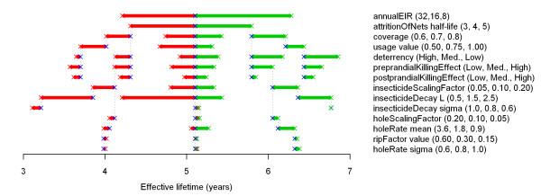
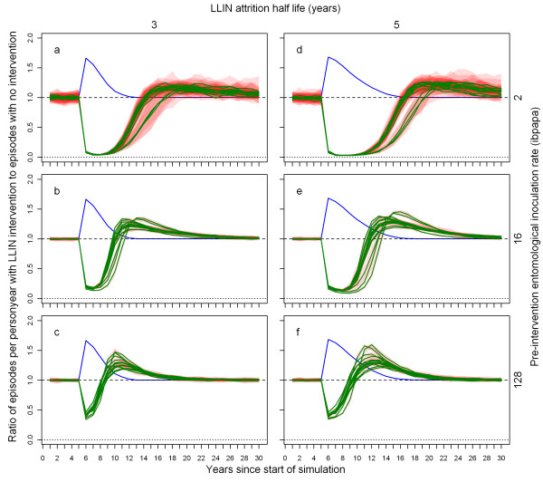
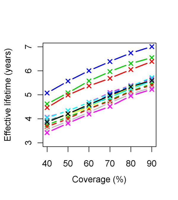
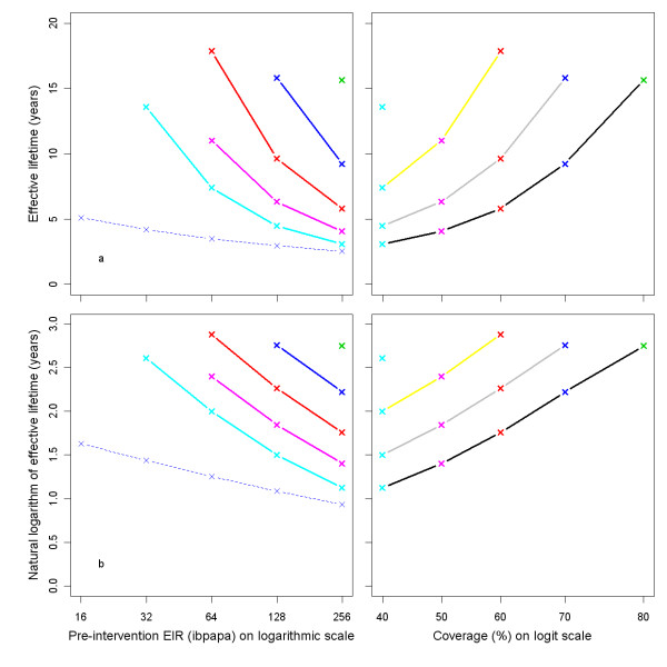
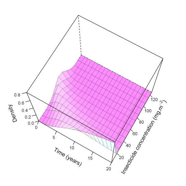
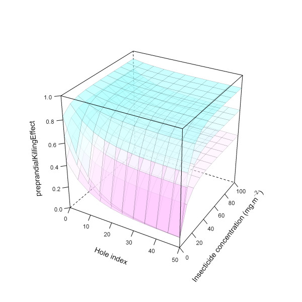
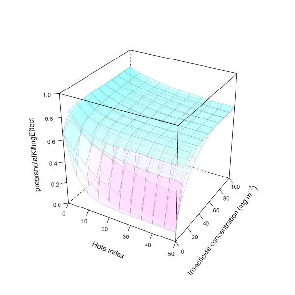
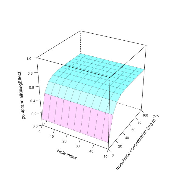
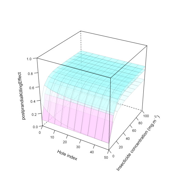
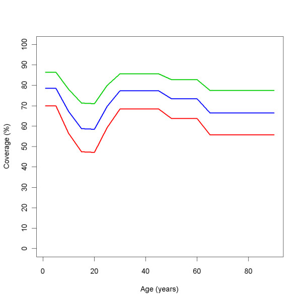
Methods: Simulation models, parameterised using available field data, were used to analyse how the distribution's effective lifetime depends on the transmission setting and on LLIN characteristics. Factors considered were the pre-intervention transmission level, initial coverage, net attrition, and both physical and chemical decay. An ensemble of 14 stochastic individual-based model variants for malaria in humans was used, combined with a deterministic model for malaria in mosquitoes.

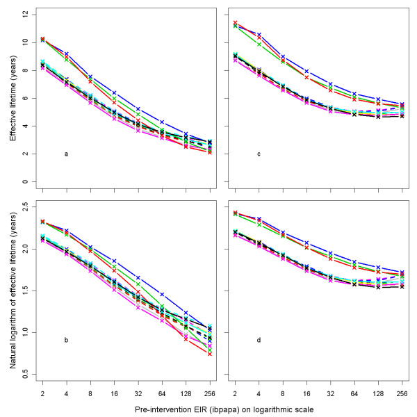
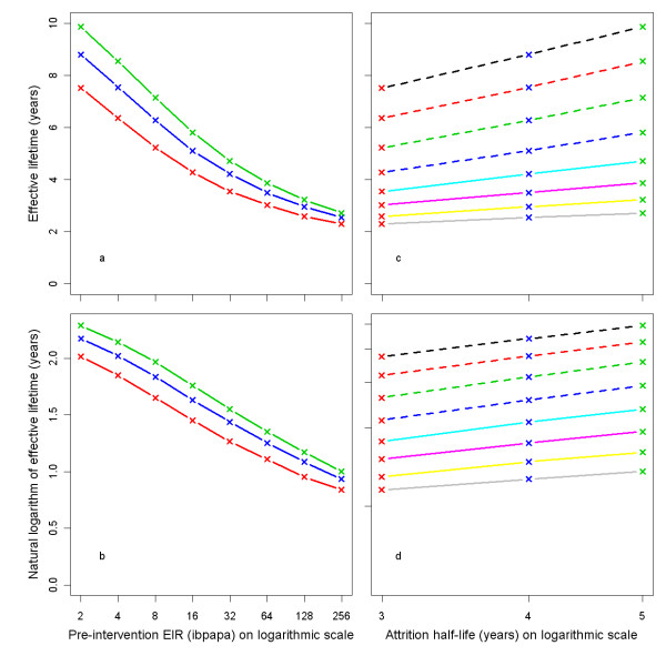
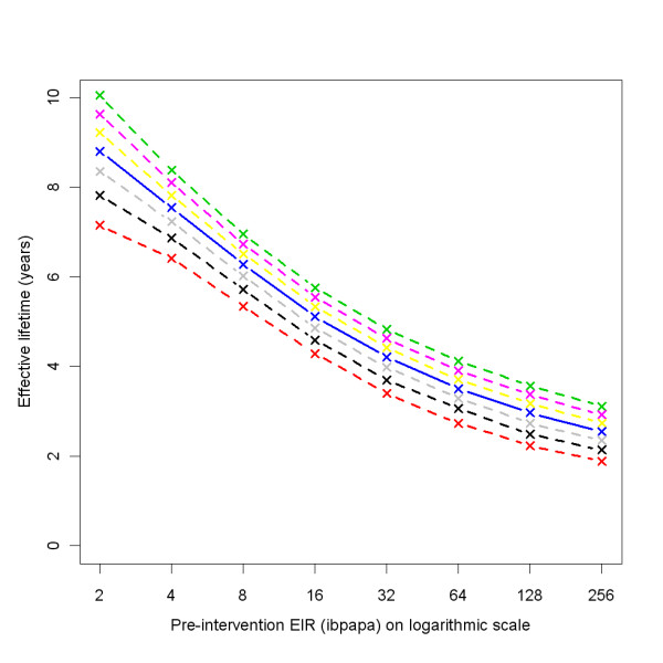
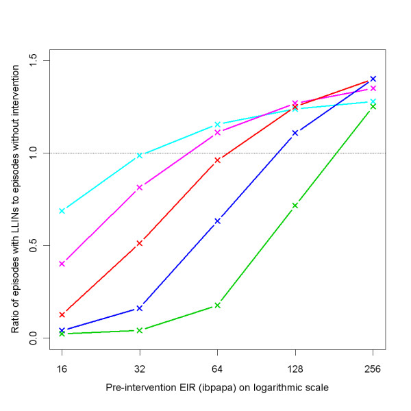
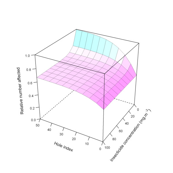
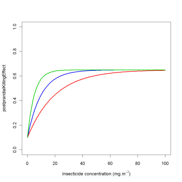
Results: The effective lifetime was most sensitive to the pre-intervention transmission level, with a lifetime of almost 10 years at an entomological inoculation rate of two infectious bites per adult per annum (ibpapa), but of little more than 2 years at 256 ibpapa. The LLIN attrition rate and the insecticide decay rate were the next most important parameters. The lifetime was surprisingly insensitive to physical decay parameters, but this could change as physical integrity gains importance with the emergence and spread of pyrethroid resistance.

Conclusions: The strong dependency of the effective lifetime on the pre-intervention transmission level indicated that the required distribution frequency may vary more with the local entomological situation than with LLIN quality or the characteristics of the distribution system. This highlights the need for malaria monitoring both before and during intervention programmes, particularly since there are likely to be strong variations between years and over short distances. The majority of SSA's population falls into exposure categories where the lifetime is relatively long, but because exposure estimates are highly uncertain, it is necessary to consider subsequent interventions before the end of the expected effective lifetime based on an imprecise transmission measure.

Figure 1

'Skeleton' diagram of model parameters. For each parameter or parameter group listed, the outcome (effective lifetime of a mass LLIN distribution, in years) depending on the parameter value is plotted on the horizontal axis. The effective lifetime was defined as the length of the period since mass distribution that the number of prevented episodes was above half the value for the year with maximum impact (i.e. the year with the minimum number of episodes), as compared to a scenario without any intervention. For each parameter, three values were chosen (listed in parenthesis after the parameter name), which represent roughly the lower, central, and upper values of the plausible parameter range. The central value is not necessarily the mean of the extreme values. These parameter values are listed in order of effect on the outcome; the first parameter value has the lowest associated outcome value, the last parameter has the highest. Crosses represent models; identical models are connected with dotted black vertical lines. Blue crosses indicate models with the central parameter value listed, green crosses indicate models with an extreme parameter value with an associated high outcome, and red crosses indicate models with an extreme parameter value with an associated low outcome. Red lines connect red and blue crosses, green lines connect blue and green crosses. In addition to results from models that vary only the parameter value in question (the other parameters taking the central value), outcomes for selected parameter combinations, often contingent on each other, where the selected parameters all have the values with the lower (red crosses), or higher (green crosses) associated outcomes are plotted.

Figure 2

Central scenario simulation with base model. a) The blue line (on left vertical axis) represents the proportion of the population covered, the red line (on left vertical axis) represents the mean insecticide in the remaining LLINs as a proportion of its initial value. The light green line (on the right vertical axis) represents the mean hole index in the remaining LLINs. b) The black line represents the number of episodes per person per five-day period. The dark green line represents the 1 year moving average of the number of episodes per person per five-day period. The red arrow indicates the approximate length of the effective lifetime of the LLIN distribution.

Figure 3

Ratio of episodes per year with LLIN mass distribution to episodes with no intervention, depending on pre-intervention EIR, attrition half-life and model variant. Each green line represents the median number of episodes of 10 simulation runs (each with unique random seed) with LLINs distributed to 70% of the people (population size = 10,000) at the beginning of year 6, the number of episodes in each intervention simulation run divided by the number of episodes in a simulation run without LLINs (also with unique random seed). Even though the values are annual totals, they are connected with lines. A column graph would be more appropriate, but less convenient for plotting multiple data series. The red semi transparent polygons represent the range of the 10 runs. Per panel, there are 14 green lines (and 14 red polygons), each representing a malaria model variant. The first column of panels (a-c) shows results for attrition with a three year half-life and the second column (d-f) for attrition with a five year half-life. The panel rows show results for pre-intervention EIRs of two (a & d), 16 (b & e), and 128 (c & f) infectious bites per adult per annum (ibpapa). Blue lines represent the proportion of people using an LLIN, added to one. Horizontal lines: dashed, ratio = 1; dotted, ratio = 0.

Figure 4

Effective lifetime of a mass LLIN distribution, depending on model variant, and pre-intervention EIR. Effective lifetime was defined as the length of the period since mass distribution during which impact on malaria episodes was above half the numerical value of the year with maximum impact (i.e. the year with the minimum number of episodes), as compared to a scenario without any intervention. Impact was measured in (a & b) all-age uncomplicated and complicated malaria episodes prevented, or (c & d) in all-age infections prevented. The entomological inoculation rate (EIR) was defined in infectious bites per adult per annum (ibpapa). Model variants [10]: R0000 = solid black lines and black crosses; R0063 = solid red lines and red crosses; R0065 = solid green lines and green crosses; R0068 = solid blue lines and blue crosses; R0111 = solid light blue lines and light blue crosses; R0115 = solid magenta lines and magenta crosses; R0121 = solid yellow lines and yellow crosses; R0125 = solid grey lines and grey crosses; R0131 = dashed black lines and black crosses; R0132 = dashed red lines and red crosses; R0133 = dashed green lines and green crosses; R0670 = dashed blue lines and blue crosses; R0674 = dashed light blue lines and light blue crosses; R0678 = dashed magenta lines and magenta crosses.

Figure 5

Effective lifetime of a mass LLIN distribution, depending on pre-intervention EIR and attrition half-life. Entomological inoculation rate (EIR) is defined as infectious bites per adult per annum (ibpapa). Attrition half-life (years): red lines and crosses = 3, blue lines and crosses = 4, green lines and crosses = 5. Figures c & d EIR: dashed black lines = 2, dashed red lines = 4, dashed green lines = 8, dashed blue lines = 16, light blue lines = 32, magenta lines = 64, yellow lines = 128, grey lines = 256. Figures a & c) Effective lifetime on vertical axis, Figures b & d) Natural logarithm of effective lifetime on vertical axis.

Figure 6

Effective lifetime of a mass LLIN distribution, depending on initial coverage and model variant. Initial coverage is the percentage of people that received access to an LLIN at the time of distribution. All parameters other than initial coverage are at central values. Model variants are coloured as indicated in Figure 4.

Figure 7

Effective lifetime of a mass LLIN distribution, depending on lifetime definition, and pre-intervention EIR. Entomological inoculation rate (EIR) is defined by infectious bites per adult per annum (ibpapa). Effective lifetime is defined as the length of the period since mass distribution during which the number of prevented all-age uncomplicated and complicated malaria episodes was above a set proportion of the numerical value of the year with maximum impact (minimum number of episodes), as compared to a scenario without any intervention, with proportions set at 0.2 (dashed green line), 0.3 (dashed magenta line), 0.4 (dashed yellow line), 0.5 (solid blue line), 0.6 (dashed grey line), 0.7 (dashed black line), or 0.8 (dashed red line).

Figure 8

Ratio of annual episodes in a situation with LLIN sustained coverage without attrition or decay to a situation without LLINs, depending on pre-intervention EIR and coverage. Each green line represents the median number of episodes of 10 simulation runs (each with unique random seed) with LLINs distributed to the people (population size = 10,000) at the beginning of year 6, the number of episodes in each intervention simulation run divided by the number of episodes in a simulation run without LLINs (also with unique random seed). The red semi transparent polygons represent the range of the 10 runs. Per panel, there are 14 green lines (and 14 red polygons), each representing a malaria model variant. The first column of panels (a-c) shows results for 60% coverage and the second column (d-f) for 80% coverage. The panel rows show results for pre-intervention EIRs of 16 (a & d), 32 (b & e), and 256 (c & f) ibpapa. Blue lines represent the proportion of people using an LLIN, added to one. Horizontal lines: dashed, ratio = 1; dotted, ratio = 0.

Figure 9

Effective lifetime of LLIN sustained coverage, depending on pre-intervention EIR and coverage. Entomological inoculation rate (EIR) is defined by infectious bites per adult per annum (ibpapa). Coverage (%): light-blue lines and crosses = 40, magenta lines and crosses = 50, red lines and crosses = 60, blue lines and crosses = 70, green crosses = 80. Figures c & d EIR: yellow lines = 64, grey lines = 128, black lines = 256. Figures a & c) Effective lifetime on vertical axis, Figures b & d) Natural logarithm of effective lifetime on vertical axis. For comparison, the effective life of a mass distribution with 70% coverage and a half life of four years is plotted in a and b (thin dashed blue lines and crosses).

Figure 10

Equilibrium ratio of episodes with LLIN sustained coverage to episodes without intervention, depending on pre-intervention EIR and coverage. Coverage (%): light blue (40), magenta (50), red (60), blue (70), green (80). The dotted horizontal line indicates a ratio of 1.

Figure 11

Distribution of the number of holes after seven years, depending on holeRate mean. The black line represents a normalised outline histogram showing the density function of the number of holes as counted by Tami and colleagues [29] in 100 nets. The coloured lines represent the normalised histogram mid-points of the number of holes in simulated nets depending on the holeRate mean, which is varied over 0.9 (green), 1.8 (blue) and 3.8 (red), with a constant holeRate sigma (see below) of 0.80.

Figure 12

Distribution of the number of holes after seven years, depending on holeRate sigma. The black line represents a normalised outline histogram showing the density function of the number of holes as counted by Tami and colleagues [29] in 100 nets. The coloured lines represent the normalised histogram mid-points of the number of holes in simulated nets depending on the holeRate sigma, which is varied over 0.6 (green), 0.8 (blue) and 1.0 (red), with a constant holeRate mean (see above) of 1.8.

Figure 13

Mean hole index over time as a function of the ripFactor value. Coloured lines plotted on the right hand vertical axis represent the mean hole index depending on the ripFactor value, which was varied over 0.6 (green), 0.3 (blue) and 0.15 (red), with all other parameters at central values. The dark blue line plotted on the left hand vertical axis represents the percentage of nets with one or more holes.

Figure 14

Mean percentage insecticide remaining over time as a function of insecticideDecay L. The coloured lines represent the insecticide remaining over time, as a percentage of the initial concentration, depending on the insecticideDecay L, which is varied over 0.5 (red), 1.5 (blue) and 2.5 (green), with a insecticideDecay sigma at the central value of 0.8 (solid lines), or at 0 (dotted lines).

Figure 15

Percentage insecticide remaining over time with all parameters at central values. The grey polygon represents the interquartile range, the solid blue line represents the median and the dashed blue line represents the mean.

Figure 16

Distribution of the percentage insecticide remaining of the initial concentration, after 38 months, depending on insecticideDecay L and insecticideDecay sigma. The coloured lines represent the normalised outline histogram of insecticide remaining as a percentage of the initial concentration in simulated nets depending on the insecticideDecay sigma, which is varied over 1.0 (green), 0.8 (blue) and 0.6 (red), and on insecticideDecay L, which is varied over 0.5 (a), 1.5 (b) and 2.5 (c).

Figure 17

Density of insecticide concentration over time, with all parameters at central values. Three dimensional plot with the proportional distribution (density) of nets over categories of insecticide concentration in 10 mg.m^-2 intervals, with lines at category mid-points. At time zero, the insecticide concentration is Gaussian distributed over the nets with mean 68.4 and standard deviation 14, but as the insecticide decays over time, the distribution is no longer Gaussian due to heterogeneity in the insecticideDecay rate. After 20 years, 77% of the nets has a concentration of 0-10 mg.m^-2.

Figure 18

Percentage of LLINs remaining over time. The coloured lines represent the LLINs remaining over time after a mass distribution, as a percentage of the initial number, depending on the attritionOfNets L, which is varied over 15.579, 20.773 and 25.966, with half-lives of 3 (red), 4 (blue) and 5 (green) years, respectively. Solid lines are for the percentage of nets with as denominator the number of people remaining in the population cohort that initially received LLINs. Dashed lines are for the percentage of nets with as denominator the total (growing) population, presuming an initial coverage of 100%.

Figure 19

Flowchart of the mosquito gonotrophic cycle. Yellow rectangles represent physical states that a mosquito can be in. Blue ovals represent phases that mosquitoes go through to reach a new state. Thin black arrows connect phases (ovals) to resulting states (yellow rectangles). Arrow annotation refers to probabilities as described by Chitnis and colleagues [8]. Purple rectangles represent states of mosquitoes as typically recorded in experimental hut studies: unfed alive (UA); unfed dead (UD); fed alive (FA); fed dead (FD); 'Trans' denotes a transitory state (not an end state as observed in mosquito counts the mornings of experimental hut studies).

Figure 20

Modelled relationship between relative number of affected mosquitoes and insecticide concentration and hole index for the 'medium' deterrency level. In this figure, insecticide concentration is varied between 0 and 100 mg.m^-2, and the hole index is varied between 0 and 50. The scaling factor for holes and insecticide (holeScalingFactor and insecticideScalingFactor, respectively), are both set to 0.10.

Figure 21

Modelled relationship between relative number of affected mosquitoes and insecticide concentration and hole index, depending on deterrency level. In this figure, insecticide concentration is varied between 0 and 100 mg.m^-2, and the hole index is varied between 0 and 50. The scaling factor for holes and insecticide (holeScalingFactor and insecticideScalingFactor, respectively), are both set to 0.10. Top layer: low deterrency; middle layer: medium level deterrency, bottom layer: high deterrency.

Figure 22

Relationship of Anopheles mortality in WHO cone tests with deltamethrin concentration, and modelled relationship. Black circles represent observations adapted from Figure 4A, page 40, in the report of the twelfth WHOPES working group meeting [34]. The coloured lines represent modelled relationship mortality = 1 - exp(-p×insecticideScalingFactor) with p the insecticide concentration and with values for insecticideScalingFactor of 0.05 (red), 0.1 (blue) and 0.2 (green).

Figure 23

Modelled relationship between relative number of affected mosquitoes and insecticide concentration and hole index for the 'medium' deterrency level, depending on holeScalingFactor and insecticideScalingFactor. In this figure, insecticide concentration is varied between 0 and 100 mg.m^-2, and the hole index is varied between 0 and 50. The scaling factor for holes and insecticide (holeScalingFactor and insecticideScalingFactor, respectively), are both set to 0.20 (top layer), 0.10 (middle layer), and 0.05 (bottom layer).

Figure 24

Modelled relationship between preprandialKillingEffect and insecticide concentration and hole index for the 'medium' preprandial KillingEffect level. In this figure, insecticide concentration is varied between 0 and 100 mg.m^-2, and the hole index is varied between 0 and 50. The scaling factor for holes and insecticide (holeScalingFactor and insecticideScalingFactor, respectively), are both set to 0.10.

Figure 25

Modelled relationship between preprandialKillingEffect and insecticide concentration and hole index, depending on preprandialKillingEffect level. In this figure, insecticide concentration is varied between 0 and 100 mg.m^-2, and the hole index is varied between 0 and 50. The scaling factor for holes and insecticide (holeScalingFactor and insecticideScalingFactor, respectively), are both set to 0.10. Top layer: high preprandialKillingEffect; middle layer: medium level preprandialKillingEffect, bottom layer: low preprandialKillingEffect.

Figure 26

Modelled relationship between preprandialKillingEffect and insecticide concentration and hole index for the 'medium' preprandialKillingEffect level, depending on hole scaling factor and insecticide scaling factor. In this figure, insecticide concentration is varied between 0 and 100 mg.m^-2, and the hole index is varied between 0 and 50. The scaling factor for holes and insecticide (holeScalingFactor and insecticideScalingFactor, respectively), are both set to 0.20 (top layer), 0.10 (middle layer), and 0.05 (bottom layer).

Figure 27

Modelled relationship between pre-prandial killing and insecticide concentration and hole index for the 'medium' postprandialKillingEffect level. In this figure, insecticide concentration is varied between 0 and 100 mg.m^-2, and the hole index is varied between 0 and 50. The scaling factor for holes and insecticide (holeScalingFactor and insecticideScalingFactor, respectively), are both set to 0.10.

Figure 28

Modelled relationship between postprandialKillingEffect and insecticide concentration and hole index, depending on postprandialKillingEffect level. In this figure, insecticide concentration is varied between 0 and 100 mg.m^-2, and the hole index is varied between 0 and 50. The scaling factor for holes and insecticide (holeScalingFactor and insecticideScalingFactor, respectively), are both set to 0.10. Top layer: high postprandialKillingEffect; middle layer: medium level postprandialKillingEffect, bottom layer: low postprandialKillingEffect.

Figure 29

Modelled relationship between the postprandialKillingEffect and insecticide concentration for the 'medium' postprandialKillingEffect level, depending on insecticide scaling factor. In this figure, insecticide concentration is varied between 0 and 100 mg.m^-2. The scaling factor for insecticide (insecticideScalingFactor), is set to 0.20 (green line), 0.10 (blue line), and 0.05 (red line).

Figure 30

Coverage depending on age. The coloured lines represent the LLIN coverage (use) directly after a mass distribution, depending on age, at 60 (red), 70 (blue) and 80 (green) average coverage, with the population structure used in the simulations (see Additional file 1).

References

1. WHO Global Malaria Programme. World Malaria Report 2010. Geneva: World Health Organization; 2010.
1. Control of Neglected Tropical Diseases WHO Pesticide Evaluation Scheme, Global Malaria Programme Vector Control Unit. Guidelines for monitoring the durability of long-lasting insecticidal mosquito nets under operational conditions. Geneva: World Health Organization; 2011. WHO/HTM/NTD/WHOPES/2011.5.
1. Kilian A. How long does a long-lasting insecticidal net last in the field? Public Health Journal. 2010;21:43–47.
1. Hawley WA, Phillips-Howard P, ter Kuile F, Terlouw DJ, Vulule JM, Ombok M, Nahlen B, Gimnig JE, Kariuki SK, Kolczak MS, Hightower AW. Community-wide effects of permethrin-treated bed nets on child mortality and malaria morbidity in western Kenya. Am J Trop Med Hyg. 2003;68(Suppl. 4):121–127. - PubMed
1. Killeen GF, Smith TA. Exploring the contributions of bed nets, cattle, insecticides and excitorepellency to malaria control: a deterministic model of mosquito host-seeking behaviour and mortality. Trans R Soc Trop Med Hyg. 2007;101:867–880. doi: 10.1016/j.trstmh.2007.04.022. - DOI - PMC - PubMed
Publication types