Controlling airborne cues to study small animal navigation

Abstract

Small animals such as nematodes and insects analyze airborne chemical cues to infer the direction of favorable and noxious locations. In these animals, the study of navigational behavior evoked by airborne cues has been limited by the difficulty of precisely controlling stimuli. We present a system that can be used to deliver gaseous stimuli in defined spatial and temporal patterns to freely moving small animals. We used this apparatus, in combination with machine-vision algorithms, to assess and quantify navigational decision making of Drosophila melanogaster larvae in response to ethyl acetate (a volatile attractant) and carbon dioxide (a gaseous repellant).

Figure 1. Apparatus design and performance

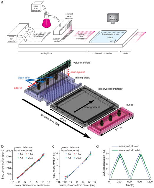
(a) Apparatus design. The upper image shows a schematic of the device. Clean airflow is regulated by a mass flow controller (MFC) into the rear of the apparatus. For EtAc experiments as shown, a second MFC controls airflow through a bubbler containing EtAc. Odorized air is injected into points across the laminar airflow within a mixing block using a solenoid valve manifold. The laminar airflow odorized with a spatial gradient of EtAc in the mixing block then passes into an observation chamber containing an experimental arena with transparent ceiling, allowing visualization of animal behavior inside the arena with a CCD camera. (Lower) Semi-transparent isometric projection of custom machined components of the apparatus, including solenoid valve manifold (green), mixing block (purple), experimental arena and observation chamber (grey), and outlet (pink). The direction of air flow (y-axis) is indicated, as is the direction of the gradient (x-axis). The odor gradient arrow points to higher concentration in the experiments described in the text.(b–c) The plots show direct measurement of the precision of linear spatial gradients of EtAc (b) or CO₂ (c) within the experimental arena. Gas concentration was measured at specific points in the experimental arena across the airflow (x-axis) at different distances from the inlet to the arena (y-axis). (d) Measurement of CO₂ concentration at inlet and outlet during a 10 minute temporal triangle ramp from 0 to 5% concentration.

Figure 2. Response to Spatial Gradients

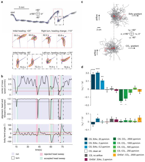
(a) Image sequence of a wild-type second instar larva crawling from left to right over 80 seconds (upper). Blue dots represent the midpoint of the larva every 200 ms. Still frames (lower) highlight two turns in which the larva achieves heading changes. Red and yellow lines indicate the contour and midline of the larva. (b) Metrics derived from the track show in (a) and used to determine behavioral state over time. The dotted and dashed boxes outline the times for the corresponding frames shown in (a). Horizontal lines are hysteretic thresholds for run determination (top panel), threshold for run determination (middle panel) and hysteretic thresholds for head sweep determination (bottom panel). (c) Trajectories (40 selected for each condition) of larvae navigating linear gradients of EtAc (top, 2 ppm/cm) and CO₂ (bottom, 2500 ppm/cm). Trajectories are displaced to start at the same point (red dot). Single trajectories are highlighted in red. (d) Navigational indices for wild-type and mutant larvae navigating gradients of varying concentrations of EtAc and CO₂ as indicated. Error bars represent standard error. +++/−−−, ++/−− reject the hypothesis that the navigation index is closer to 0 than +/−0.1, +/− 0.05 respectively at p < 0.01 using one tailed t-test, * rejects the hypothesis that the navigation index is 0 at p < 0.01 using two tailed t-test.

Figure 3. Navigation of a 2ppm/cm Ethyl Acetate concentration gradient

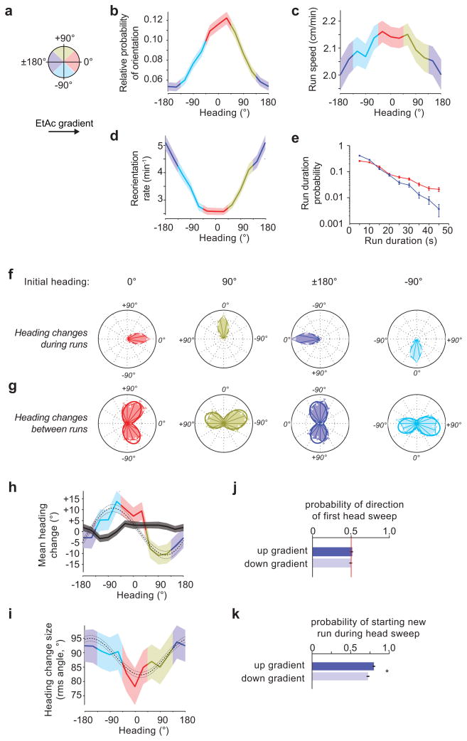
For the data in this figure,10 experiments, 202 animals and 290 hours of behavior were analyzed. (a) The schematic depicts heading angles. 0° is towards higher concentration. (b) Relative probability of headings during runs. (c) Speed vs. heading during runs. (d) Turn rate vs. heading. (e) Durations of runs headed up (red, 1537 runs) or down gradients (blue, 1091 runs) (f) Heading changes during runs sorted by initial run direction: up gradients (red, 1499 runs), down gradients (blue, 1062 runs), orthogonal with higher concentration to the right (gold, 1354 runs), and orthogonal with higher concentration to the left (cyan, 1184 runs) (g) Heading changes achieved by turns, sorted, as in (f), on the basis of heading immediately prior to the turn (0° - 1201 reorientations; 180° - 1105 reorientations; 90° - 1214 reorientations; −90° - 1049 reorientations), (h) mean heading change achieved by runs (black line) and turns (colored line) vs. initial heading/heading prior to turn. (i) RMS turn angle vs. run heading prior to turn. The dashed and dotted lines in (e) and (f) represent the prediction and 95% confidence interval of the model described in methods. (j,k) Statistics of head sweeps during turns after runs headed orthogonal to the concentration gradient. The plots show probability of direction of the first head sweep (j) (1967 head sweeps) and probability that the larva initiates a new run during head sweeps (k) (2341 head sweeps). * rejects the hypothesis that the probabilities are the same at p<0.01 using Welch’s t-test. error bars and regions: (b,c) s.e.m. calculated as described in the methods, (d,e,f,g,j,k) s.e. derived from counting statistics (h,i) s.e.m.

Figure 4. Navigation of a 2500 ppm/cm Carbon dioxide concentration gradient

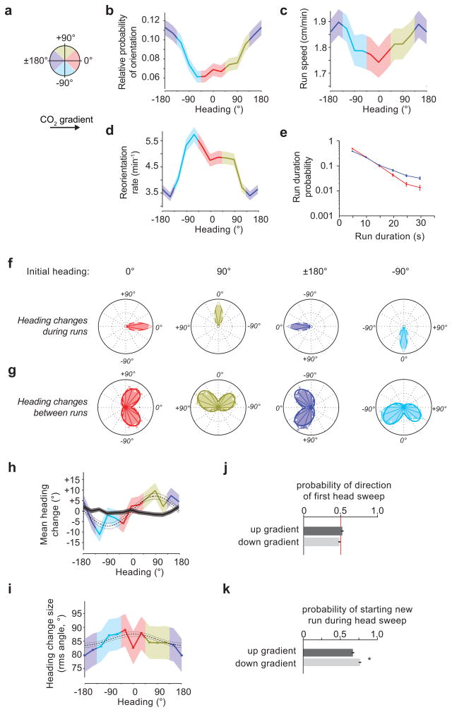
For the data in this figure, 21 experiments, 168 animals, 31 hours of behavior were analyzed. (a) The schematic depicts heading angles. 0° is towards higher concentration. (b) Relative probability of headings during runs. (c) Speed vs. heading during runs. (d) Turn rate vs. heading. (e) Durations of runs headed up (red, 1494 runs) or down gradients (blue, 1866 runs) (f) Heading changes during runs sorted by initial run direction: up (red, 1484 runs), down gradients (blue, 1844 runs), orthogonal with higher concentration to the right (gold, 1651 runs), and orthogonal with higher concentration to the left (cyan, 1664 runs) (g) Heading changes achieved by turns, sorted, as in (f), on the basis of heading immediately prior to the turn (0° - 1196 reorientations; 180° - 1336 reorientations; 90° - 1306 reorientations; −90° - 1375 reorientations), (h) mean heading change achieved by runs (black line) and turns (colored line) vs. initial heading/heading prior to turn. (i) RMS turn angle vs. run heading prior to turn. The dashed and dotted lines in (e) and (f) represent the prediction and 95% confidence interval of the model described in methods. (j,k) Statistics of head sweeps during turns after runs headed orthogonal to the concentration gradient. The plots show probability of direction of the first head sweep (j) (2497 head sweeps) and probability that the larva initiates a new run during head sweeps (k) (3254 head sweeps). * rejects the hypothesis that the probabilities are the same at p<0.01 using Welch’s t-test. error bars and regions: (b,c) s.e.m. calculated as described in the methods, (d,e,f,g,j,k) s.e. derived from counting statistics (h,i) s.e.m.

Figure 5. Temporal CO₂ and EtAc gradients

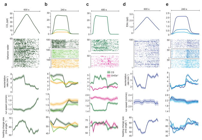
Statistics of turning decisions of larvae subjected to spatially uniform temporal gradients of CO₂ delivered as repeating cycles of triangle waves (a) and steps (b,c) and of EtAc delivered as triangle waves (d) and steps (e). Upper panel in each plot shows one cycle of stimulus waveform. Raster plots indicate periods in which an individual larva was turning during the cycle, each row represents one larva tracked continuously through a cycle (a, n = 65, b n = 100 ea condition, c n = 50 ea condition, d,e n = 100 each condition) Lower panels show the turning rate and s.e. derived from counting statistics, mean crawling speeds and s.e.m. calculated as described in methods, and mean square heading change after turns and one s.e. vs. the time within each cycle. Data from wild-type larvae (Canton-S) are shown in (a,b,d and e). The step response of wild-type larvae and GR63a¹ mutant larvae are compared in (c).

References

-
- Brody CD, Hopfield JJ. Simple networks for spike-timing-based computation, with application to olfactory processing. Neuron. 2003;37:843–852. - PubMed
- Cleland TA, Linster C. Computation in the olfactory system. Chem Senses. 2005;30:801–813. - PubMed
- Chalasani SH, et al. Dissecting a circuit for olfactory behaviour in Caenorhabditis elegans. Nature. 2007;450:63–70. - PubMed
- Masse NY, Turner GC, Jefferis GS. Olfactory information processing in Drosophila. Curr Biol. 2009;19:R700–13. - PubMed
Publication types
MeSH terms
Substances
Grants and funding
LinkOut - more resources
Full Text Sources
Molecular Biology Databases