Review
. 2010:3:169-208.
doi: 10.1109/RBME.2010.2084567.

Retinal imaging and image analysis

Affiliations
Review

Retinal imaging and image analysis

Michael D Abràmoff et al. IEEE Rev Biomed Eng. 2010.

Abstract

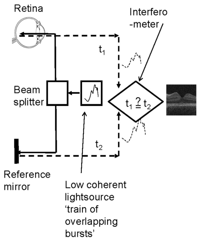
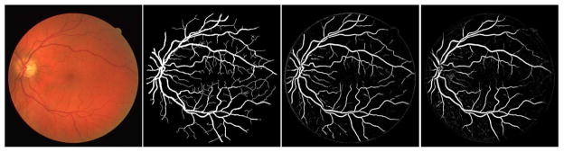
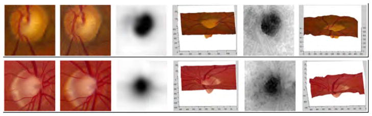
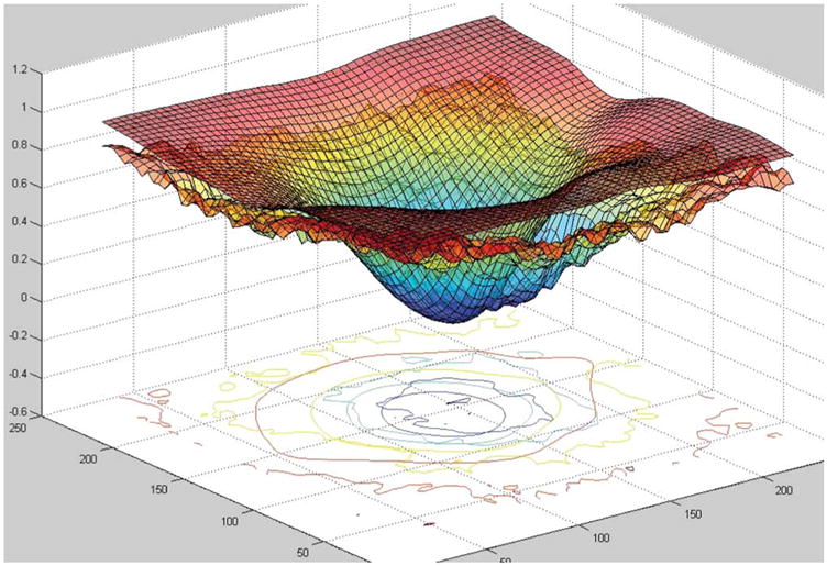
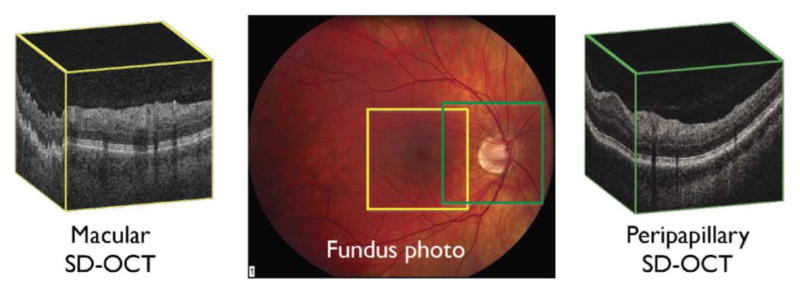
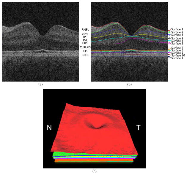
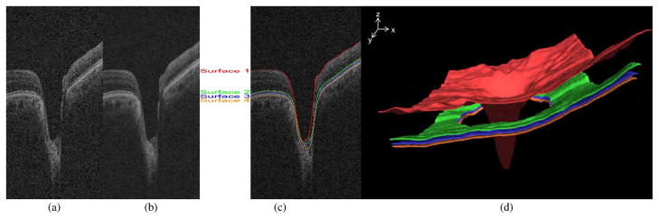
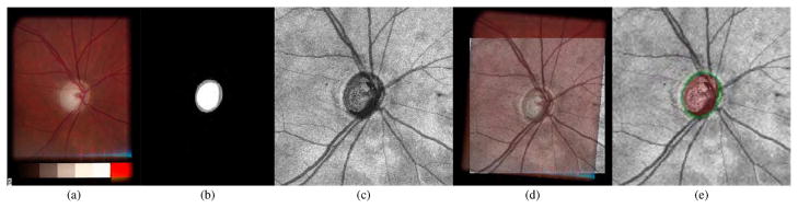
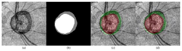
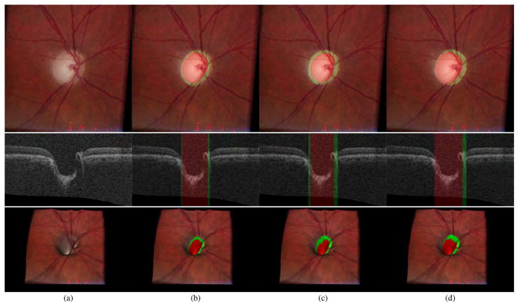
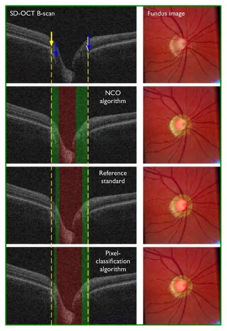
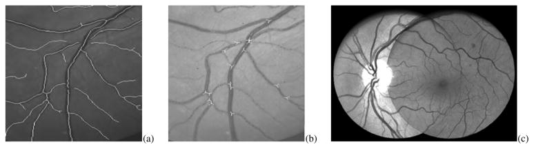
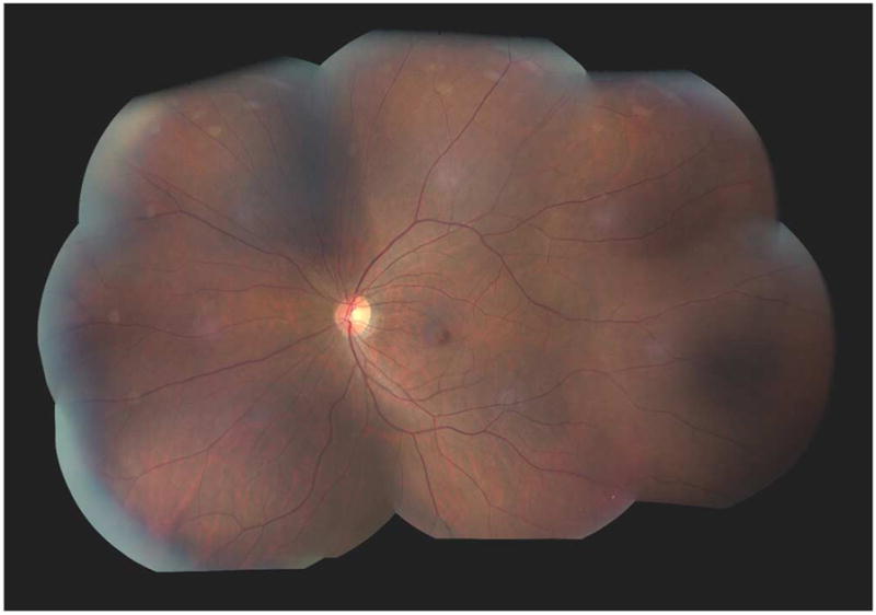
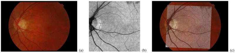
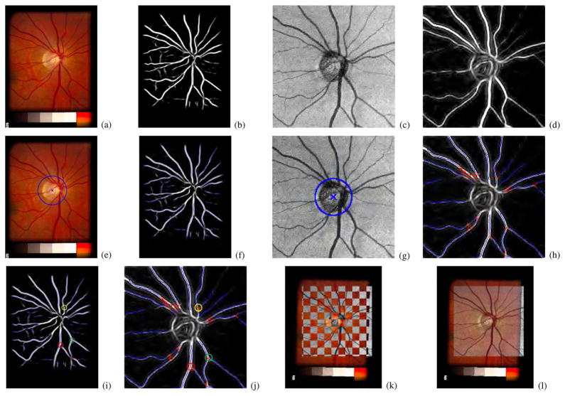
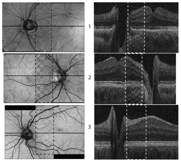
Many important eye diseases as well as systemic diseases manifest themselves in the retina. While a number of other anatomical structures contribute to the process of vision, this review focuses on retinal imaging and image analysis. Following a brief overview of the most prevalent causes of blindness in the industrialized world that includes age-related macular degeneration, diabetic retinopathy, and glaucoma, the review is devoted to retinal imaging and image analysis methods and their clinical implications. Methods for 2-D fundus imaging and techniques for 3-D optical coherence tomography (OCT) imaging are reviewed. Special attention is given to quantitative techniques for analysis of fundus photographs with a focus on clinically relevant assessment of retinal vasculature, identification of retinal lesions, assessment of optic nerve head (ONH) shape, building retinal atlases, and to automated methods for population screening for retinal diseases. A separate section is devoted to 3-D analysis of OCT images, describing methods for segmentation and analysis of retinal layers, retinal vasculature, and 2-D/3-D detection of symptomatic exudate-associated derangements, as well as to OCT-based analysis of ONH morphology and shape. Throughout the paper, aspects of image acquisition, image analysis, and clinical relevance are treated together considering their mutually interlinked relationships.


Figures

Fig. 1
Fig. 1
First known image of human retina as drawn by Van Trigt in 1853 [1].
Fig. 2
Fig. 2
Illustration of eye anatomy and retinal layers [2], [3]. (a) Cross-sectional view of eye and its major structures. Retina is a thin transparent tissue that lines the back of the eye and is comprised of a number of layers, as illustrated in enlarged portion. (b) Schematic drawing of cellular layers of retina. (a) Two-dimensional illustration of eye anatomy. (b) Schematic of retinal layers. Illustrations from Kolb [3] used with kind permission of Sigma Xi, The Scientific Research Society, Research Triangle Park, NC.
Fig. 3
Fig. 3
Early drawing of retinal vasculature including outlines of ONH and fovea published by Purkyne in 1823 [30].
Fig. 4
Fig. 4
Schematic diagram of OCT, with emphasis on splitting of the light, overlapping train of labeled bursts based on their autocorrelogram, and their interference after being reflected from retinal tissue as well as from the reference mirror (assuming the time delays of both paths are equal).
Fig. 5
Fig. 5
Automated vessel analysis. From left to right: fundus image; retinal specialist annotation; vesselness map from Staal algorithm [76]; vesselness map from direct pixel classification [73].
Fig. 6
Fig. 6
Automated analysis of fundus photographs. (a) Fundus photograph showing several lesions typical of diabetic retinopathy. (b) Detection of red lesions (RL)—microaneurysms and hemorrhages. (c) Detection of bright lesions (BL)—lipoprotein exudates. (d) Detection of neovascularization (NVD) of the optic disc. (e) All automatically detected lesions shown.
Fig. 7
Fig. 7
Typical steps necessary for analysis of fundus images, in this case for early diabetic retinopathy. Top row from left to right: original image; detection of fovea and optic disc superimposed as yellow circles on the vesselness map; automatically detected red lesions indicated in shades of green, bright lesions in shades of blue. Bottom row: details of red and bright lesion detection steps shown in a small region of the image including pixel classification identifying suspect pixels, clustering of suspect pixels, and classification of clusters as lesions.
Fig. 8
Fig. 8
Red lesion pixel feature classification. (a) Part of green color plane of a fundus image. Shown are pieces of vasculature and several red lesions. Bright lesions called exudates are also a symptom of DR. Circles mark location of some of the red lesions in the image. (b) After subtracting median filtered version of the green plane large background gradients are removed. (c) All pixels with a positive value are set to zero to eliminate bright lesions in the image. Note that exudates often partially occlude red lesions. Non-occluded parts of red lesions show up clearly in this image. An example of this is marked with a rectangle. (d) Pixel classification result produced by contrast enhancement step. Non-occluded parts of hemorrhages are visible together with the vasculature and a number of red lesions.
Fig. 9
Fig. 9
Red lesion detection. (a) Thresholded probability map. (b) Remaining objects after connected component analysis and removal of large vasculature. (c) Shape and size of extracted objects in panel (b) does not correspond well with actual shape and size of objects in original image. Final region growing procedure is used to grow back actual objects in original image which are shown here. In (b) and (c), the same red lesions as in Fig. 8(a) are indicated with a circle.
Fig. 10
Fig. 10
Bright lesion detection algorithm steps performed to detect and differentiate “bright lesions.” From left to right: exudates, cotton-wool spots, and drusen. From top to bottom: relevant regions in the retinal color image (all at same scale); a posteriori probability maps after first classification step; pixel clusters labeled as probable bright lesions (potential lesions); bottom row shows final labeling of objects as true bright lesions, overlaid on original image.
Fig. 11
Fig. 11
Registration of fundus image pair using (a) quadratic model and (b) RADIC model. Vessel center lines are overlaid for visual assessment of registration accuracy. This registration is performed to disk-centered and macula-centered images to provide an increased anatomic field of view.
Fig. 12
Fig. 12
Registration of anatomic structures according to increasing complexity of registration transform—500 retinal vessel images are overlaid and marked with one foveal point landmark each (red spots). Rigid coordinate alignment by (a) translation, (b) translation and scale, and (c) translation, scale, and rotation.
Fig. 13
Fig. 13
Atlas coordinate mapping by TPS: (a) before and (b) after mapping. Naive main arch traces obtained by Dijkstra’s line-detection algorithm are drawn as yellow lines that undergo polynomial curve fitting to result in blue lines. Atlas landmarks (disc center, fovea, and vascular arch) are drawn in green, and equidistant radial sampling points marked with dots.
Fig. 14
Fig. 14
Example application of employing retinal atlas to detect imaging artifacts. (a), (c) Color fundus images with artifacts. (b), (d) Euclidean distance maps in atlas space using atlas coordinate system. Note that distances are evaluated within atlas image. Consequently, field of view of distance map is not identical to that of fundus image.
Fig. 15
Fig. 15
Annotations of optic disc stereo pair by three expert glaucoma specialists. Note substantial inter-observer variability. ONH rim is shown in grayish and cup in whitish overlay on left image of stereo pair. Rightmost panel D shows a reference standard that was created from expert analyses A, B, C by majority voting with white color representing cup, gray color denoting rim, and black color corresponding to background.
Fig. 16
Fig. 16
Color opponency steerable Gaussian filter bank kernel examples. First row, from left to right shows dark-bright opponency kernels for 0th order, first-order 0° to local gradient, first-order 90° to local gradient, second-order 0° to local gradient, second-order 60° to local gradient, and second-order 120° to local gradient, at a scale of 32 pixels. Second row, same for scale of 64 pixels, and third row for scale of 128 pixels. Next three rows show identical information for blue-yellow opponency kernels, and last three rows show red-green kernels. Smaller scales not shown because they are difficult to depict. These kernel images represent responses of each of feature detectors to an impulse function. Note that true kernel colors are shown.
Fig. 17
Fig. 17
Classification of stereo pairs (left two columns) by glaucoma specialists (third column), three glaucoma fellows (columns 4–6), and automated pixel feature classification (right-most column). Rows from top to bottom: Small, medium, large disc excavation, and excavation with inferior notching.
Fig. 18
Fig. 18
Two examples of 3-D ONH surface reconstruction obtained from a stereo fundus pair and from 3-D OCT scan shown in two rows. From left to right (both rows): left and right fundus image centered at the optic disc. Shape estimate of optic nerve head surface represented as grayscale depth maps derived from OCT scan. Reference (left) image shown to correspond to OCT scan view. Shape estimate of optic nerve surface represented as grayscale depth maps derived from stereo fundus pair analysis. Reference (left) image shown to correspond to output from stereo fundus pair reconstruction.
Fig. 19
Fig. 19
Example of 3-D agreement between stereo-fundus-photography-derived (lower surface) and OCT-derived (upper surface, smoothed) 3-D reconstructions of ONH shape.
Fig. 20
Fig. 20
Typical scanning locations (illustrated on center fundus photograph) of spectral-domain OCT scanning system: Macular volumetric scans (left, in yellow) which are centered on macula, and peripapillary volumetric scans (right, in green) which are centered on optic nerve head.
Fig. 21
Fig. 21
Segmentation results of 11 retinal surfaces (ten layers). (a) X-Z image of OCT volume. (b) Segmentation results, nerve fiber layer (NFL), ganglion cell layer (GCL), inner plexiform layer (IPL), inner nuclear layer (INL), outer plexiform layer (OPL), outer nuclear layer (ONL) + inner segments (IS), outer segments (OS), and retinal pigment epithelium complex (RPE+). Stated anatomical labeling is based on observed relationships with histology although no general agreement exists among experts about precise correspondence of some layers, especially outermost layers. (c) Three-dimensional rendering of segmented surfaces (N: nasal, T: temporal).
Fig. 22
Fig. 22
Illustration of helpfulness in using 3-D contextual information in intraretinal layer segmentation process. (Top) Sequence of 2-D result on three adjacent slices within spectral-domain volume obtained using a slice-by-slice 2-D graph-based approach. Note the “jump” in segmentation result for third and fourth surfaces in middle slice. (Bottom) Sequence of 3-D result on same three adjacent slices using same graph-based approach, but with addition of 3-D contextual information. Three-dimensional contextual information prevented third and fourth surface segmentation from failing.
Fig. 23
Fig. 23
Geometry of textural characterization of macula. Local textural or thickness indices are extracted within intersection of region-defining columns (typically with a rectangular support domain in xy plane) with each segmented intraretinal layer. Features computed in each of these intersections may be used to define an abnormality index for (x, y) line at center of the column when detecting macular lesions as described in Section V-C.
Fig. 24
Fig. 24
Example of spectral 3-D OCT vessel segmentation. (a) Vessel silhouettes indicate position of vasculature. Also indicated in red are slice intersections of two surfaces that delineate subvolume in which vessels are segmented (superficial retinal layers toward vitreous are at the bottom). (b) Two-dimensional projection image extracted from projected subvolume of spectral 3-D OCT volume. (c) Automatic vessel segmentation. (d) Vessel segmentation after postprocessing—removing disconnected pieces and connecting large segments.
Fig. 25
Fig. 25
Example 3-D vasculature segmentation result from OCT volumetric scan [158].
Fig. 26
Fig. 26
Normal appearance of three intraretinal layers (NFL, INL and OS, see Fig. 21) in feature space optimized for SEAD footprint detection. For each feature, a map of the average (standard deviation) of feature values across macula is displayed on left (right). Inertia (b) is correlated with thickness of layer (d). Note that standard deviations of wavelet coefficients (c) and entropy (e) are almost uniform (black) across macula in normal eyes. (a) Average intensity; (b) inertia (co-occurrence matrix); (c) standard deviation wavelet coefficients (level 1); (d) layer thickness; (e) entropy (co-occurrence matrix).
Fig. 27
Fig. 27
Example of SEAD footprint detection. Panel (a) presents an xz slice running through SEADs in SD-OCT volume. Expert standards for footprint of these SEADs and automatically generated SEAD footprint probability map, in xy plane, are presented in panels (b) and (c), respectively. Note probability scale in panel (c). Projection of xz slice in xy plane is represented by a vertical line in (b) and (c). Location of SEADs visible in panel (a) are indicated by vertical lines in each panel.
Fig. 28
Fig. 28
Repeatability study—two scans from same eye were acquired on same day at close temporal intervals. For each panel (a), (b), upper row shows binary SEAD footprint representing independent standard. Lower row shows SEAD footprints obtained by our automated method, gray levels represent probability of the point belonging to SEAD footprint; probability scale is provided in Fig. 27(c). These probabilities were thresholded to arrive at a binary segmentation. When varying threshold levels, obtained performance yields ROC curves discussed in text. (a) First scan and (b) second scan.
Fig. 29
Fig. 29
SEAD segmentation from 3-D OCT and SEAD development over time: top row: 0, 28, and 77 days after first imaging visit. Middle row: 0 and 42 days after first imaging visit. Bottom row: 0, 14, and 28 days after first imaging visit. Three-dimensional visualization in right column shows data from week 0. Each imaging session was associated with anti-VEGF reinjection.
Fig. 30
Fig. 30
Automated intraretinal layer segmentation approach in presence of SEADs. (a), (b) Zeiss Cirrus OCT image data—two perpendicular slices from 3-D volume. (c), (d) Automated layer/SEAD segmentation. (e) SEAD and layers in three dimensions.
Fig. 31
Fig. 31
Intraretinal surface segmentation. (a) Original ONH-centered OCT volume. (b) Smoothed OCT volume. (c) Intraretinal surface segmentation result overlaid on original OCT volume. Search space for surfaces are constrained by previously segmented surfaces in multiresolution fashion. (d) Three-dimensional rendering of four segmented intraretinal surfaces. Regions of surfaces 2, 3, and 4 around the optic nerve head were ignored since intraretinal surfaces are ambiguous in these regions.
Fig. 32
Fig. 32
Acquisition of ONH ground truth of spectral-domain OCT scan. (a) One of a pair of stereo color photographs. (b) Optic disc ground truth of (a), which is manually segmented by glaucoma expert through planimetry on one (left) of the pair of stereo fundus photographs while viewing the pair through a stereo viewer. Optic disc cup is in white, and neuroretinal rim is in gray. (c) OCT projection image. (d) Fundus photograph (panel a) registered onto OCT projection image (panel c). (e) OCT projection image overlapped with ONH ground truth. Optic disc cup is in red, and neuroretinal rim is in green.
Fig. 33
Fig. 33
Example of optic disc cup and neuroretinal rim segmentation. (a) OCT projection image. (b) Segmentation result using contextual k-NN classifier with convex hull-based fitting. (c) OCT projection image overlapped with reference standard. Optic disc cup is in red, and neuroretinal rim is in green. (d) OCT projection image overlapped with (b).
Fig. 34
Fig. 34
Example of ONH segmentation performance [unsigned error for the optic disc cup = pixels (0.038 mm) and unsigned error for the neuroretinal rim = pixels (0.026 mm)]. From top to bottom, left stereo color photograph, X-Z image at center of OCT volume and 3-D rendering of top intraretinal surface mapped with left stereo color photograph. (a) Without any overlap. (b) Overlapped with result from contextual k-NN classifier with convex hull-based fitting. Optic disc cup is in red and neuroretinal rim is in green. (c) Overlapped with reference standard. (d) Overlapped with manual segmentation from second observer.
Fig. 35
Fig. 35
Example illustration of differences between structure-based segmentation of NCO/cup on OCT, glaucoma expert definition of optic disc margin and cup from manual planimetry, and pixel-classification-based segmentation of disc/cup on OCT. From top to bottom: raw SD-OCT and corresponding fundus image (top), structure-based (row 2), expert (on fundus photography) (row 3), and pixel-classification-based (bottom) segmentations overlapping with raw SD-OCT and corresponding fundus image. From left to right: SD-OCT central B-scan (left) and fundus image (right). Yellow arrows indicate position of NCO from algorithm (with dashed yellow line indicating projected NCO position). Blue arrows indicate clinical disc margin from RS. Green and red colors indicate each method’s projected rim and cup regions, respectively [170].
Fig. 36
Fig. 36
Example of fundus retinal image registration. (a) Detail of two fundus images with detected vessel centerlines. (b) Identified vessel landmarks. (c) Example registration result achieved on two overlapping fundus images.
Fig. 37
Fig. 37
Retinal fundus image registration. Wide-angle fundus image is constructed by mutual registration of eight individual fundus photographs.
Fig. 38
Fig. 38
Registration of fundus images to 2-D OCT projection data. (a) Fundus camera image. (b) Two-dimensional projection (through depth dimension) of 3-D OCT data. (c) Registered and blended fundus-OCT images via application of affine transformation model with three identified vascular landmarks.
Fig. 39
Fig. 39
Step-by-step process of registering fundus images to 2-D OCT projection data of the same subject. (a) Color fundus image. (b) Vascular segmentation in fundus image. (c) OCT projection image. (d) Vascular segmentation in OCT projection image. (e) ONH area and ONH center detected in fundus image. (f) Vascular center lines (blue) and bifurcations (red) in fundus image—bifurcations serve as prospective landmarks for which correspondence with OCT landmarks is determined in the next step. (g) ONH area and ONH center detected in OCT projection image. (h) Vascular centerlines (blue) and bifurcations (red) in OCT image—bifurcations serve as prospective landmarks for which correspondence with fundus landmarks is determined in the next step. (i) Highest reliability OCT-fundus corresponding landmarks identified in fundus image. (j) Highest reliability OCT-fundus corresponding landmarks identified in OCT image. (k) Registered OCT-fundus image—quality of registration shown in checkerboard image. (l) Registered OCT-fundus image—averaging-based blending used to construct image.
Fig. 40
Fig. 40
Three-dimensional registration of macular and peripapillary OCT from the same subjects. Z-axis projection images of registered volumes are shown in left column. Representative depth-axis slices from volumes are shown on right to demonstrate registration performance in three dimensions. Location of displayed slice is indicated by a black line on registered projection images. Overlapping areas of scans are outlined by dashed rectangles to demonstrate that only relatively small regions of overlap existed. Within these rectangular patches, image data from both OCT images are shown intermittently in a checkerboard pattern to illustrate agreement of resulting registration. In projection images (same as in fundus photography), optic nerve head can be identified as a large dark region with vasculature emanating from that region while fovea can be identified as a small dark region centrally located in nonvascular region of the registered image.

Similar articles

Cited by

References

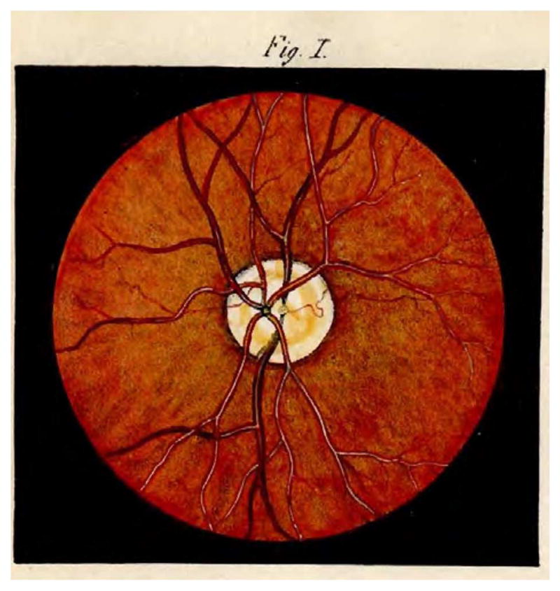
    1. Van Trigt AC. Trajecti ad Rhenum. 1853. Dissertatio ophthalmologica inauguralis de speculo oculi.
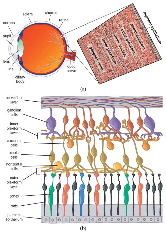
    1. Kolb H. How the retina works. Amer Scientist. 2003;91(1):28–35.
    1. Kolb H, Fernandez E, Nelson R, Jones BW. Webvision: Organization of the retina and visual system. 2005 [Online]. Available: http://webvision.med.utah.edu/ - PubMed
    1. WHO. [Online]. Available: http://www.who.int/diabetes/publications/Definitionanddiagnosisofdiabete....
    1. Nat. Eye Inst. Visual problems in the U.S. Nat Eye Inst. 2002 [Online]. Available: http://www.nei.nih.gov/eyedata/pdf/VPUS.pdf.

Publication types

MeSH terms