Modular Organization of Functional Network Connectivity in Healthy Controls and Patients with Schizophrenia during the Resting State

Abstract

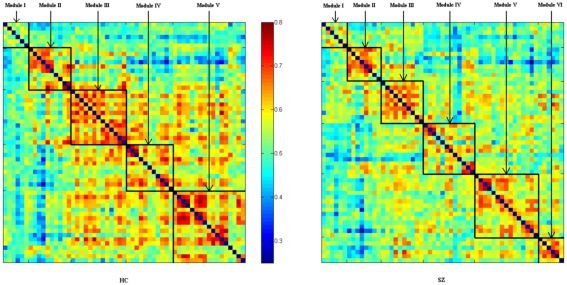
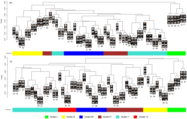
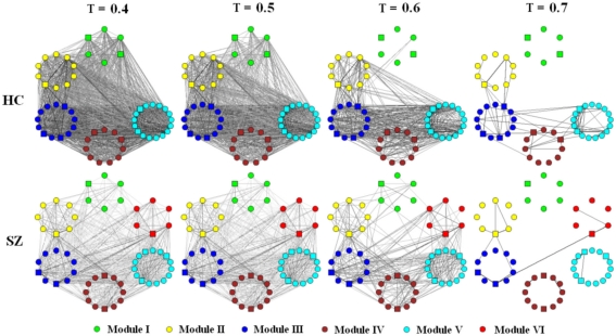
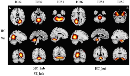
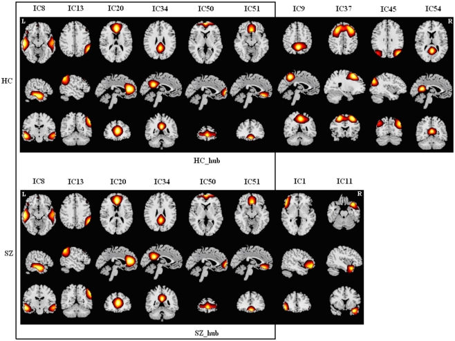
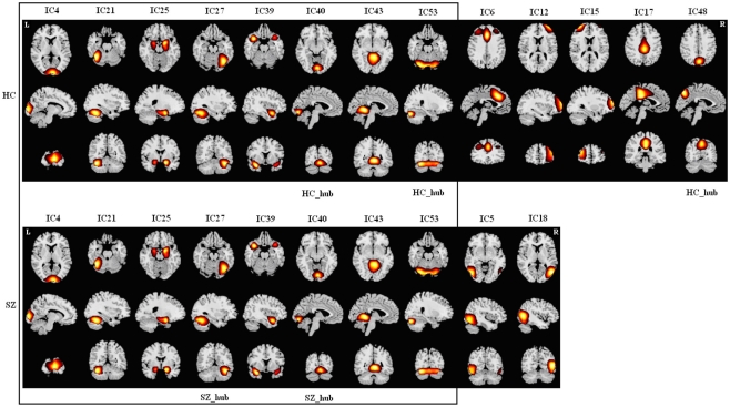
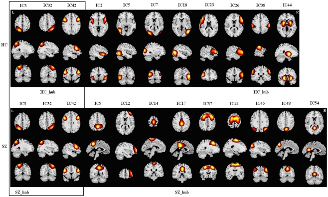
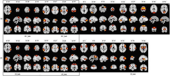
Neuroimaging studies have shown that functional brain networks composed from select regions of interest have a modular community structure. However, the organization of functional network connectivity (FNC), comprising a purely data-driven network built from spatially independent brain components, is not yet clear. The aim of this study is to explore the modular organization of FNC in both healthy controls (HCs) and patients with schizophrenia (SZs). Resting state functional magnetic resonance imaging data of HCs and SZs were decomposed into independent components (ICs) by group independent component analysis (ICA). Then weighted brain networks (in which nodes are brain components) were built based on correlations between ICA time courses. Clustering coefficients and connectivity strength of the networks were computed. A dynamic branch cutting algorithm was used to identify modules of the FNC in HCs and SZs. Results show stronger connectivity strength and higher clustering coefficient in HCs with more and smaller modules in SZs. In addition, HCs and SZs had some different hubs. Our findings demonstrate altered modular architecture of the FNC in schizophrenia and provide insights into abnormal topological organization of intrinsic brain networks in this mental illness.

Keywords: ICA; R-fMRI; functional network connectivity; modularity; schizophrenia.

Figure 1

Structure of mean signed similarity for each group after organized by modules. ICs’ index (from top to down; from left to right) is: HC, Module I (22 30 31 36 52 57), Module II (8 13 20 34 50 51 9 37 45 54), Module III (4 21 25 27 39 40 43 53 6 12 15 17 48), Module IV (3 32 42 2 5 7 18 23 26 38 44), Module V (19 24 28 33 35 47 49 55 10 16 29 46 56 1 11 14 41); SZ, Module I (22 30 31 36 52 57), Module II (8 13 20 34 50 51 1 11), Module III (4 21 25 27 39 40 43 53 5 18), Module IV (3 32 42 9 12 14 17 37 41 45 48 54), Module V (19 24 28 33 35 47 49 55 2 6 15 23 26 38 44), Module VI (10 16 29 46 56 7).

Figure 2

Dendrogram and modules found using the dynamic tree cutting algorithm in each group. Each figure shows the hierarchical structure of the FNC based on the mean signed similarity across 24 HCs or 24 SZs. Modules are labeled by colors. Numbers under maps of brain components are IC indexes as determined by the sequence of output from GIFT. Not all nodes in a same module are close to each other in the dendrogram (see Module IV and Module V of HCs for example). That is because “Dynamic Hybrid” variant which improves the detection of outlying members of each cluster was selected when performing the dynamic branch cut algorithm. In addition to information from the dendrogram, it utilizes dissimilarity information among the objects. For details of the algorithm see Langfelder et al. (2008).

Figure 3

Schematic modular architecture of FNC for each group. Nodes in a given module are placed in a small circle. To show how edges disappear with threshold (T) change, graphs (each consisted of 57 ICs) built by T at 0.4, 0.5, 0.6, and 0.7 are shown respectively. An edge (either inter- or intra-module edge) is shown in the graph if its weight bigger then T. The thicker and the darker an edge, the higher its weight. Hubs are indicated by square nodes.

Figure A1

Spatial maps (z-score maps, same in Figures A2–A6) of components in module I for HCs and SZs. Hubs of this module in each group are labeled. Each column shows one component in axial, sagittal, and coronal views. In this module, both groups have six common components including three cerebellar networks, two occipital networks, and one temporal network. We designated this module as “cerebellar–occipital module” (C–O Module). Two cerebellar components are hubs in HCs and one cerebellar component is hub in SZs.

Figure A2

Spatial maps of components in module II for HCs (upper) and SZs (lower). Hubs of each module are labeled. Each column shows one component in axial, sagittal, and coronal views. There are six common components [in the box, most of which are default mode network (DMN) areas] between the groups. This module was designated as “DMN Module.” HCs have another four networks which are also loosely characterized as DMN regions, whereas SZs have another two networks including one frontal component and one temporal component. HCs and SZs have the common frontal hub in this module.

Figure A3

Spatial maps of components in module III for HCs (upper) and SZs (lower). Hubs of this module in each group are labeled. Each column shows one component in axial, sagittal, and coronal views. There are eight common components (in the box) including three occipital components, three cerebellar components, one parahippocampal component, and one temporal component. HCs have five additional components including two frontal components, two cingulum components, and one precuneus component. SZs have two additional components including one occipital component and one temporal component. As the components of this module in HCs represent regions distributed across almost the whole brain, we designated this module as “Global Module” (G1 Module). There are three hubs in HCs and two hubs in SZs.

Figure A4

Spatial maps of components in module IV for HCs (upper) and SZs (lower). Hubs of this module in each group are labeled. Each column shows one component in axial, sagital, and coronal views. There are three common components (in the box) including two parietal components and one frontal component. HCs have another eight components including two frontal components, two occipital components, one temporal component, one central component, one putamen component, and one temporal-frontal component. SZs have another nine components including three frontal components, three precuneus component, one angular component, one cingulum component, and one central component. As most of the components of this module in HCs are from attention network, we designated this module as “Attention Module” (A Module). There are two different hubs in this module for the two groups.

Figure A5

Spatial maps of components in module V for HCs (upper) and SZs (lower). Hubs of this module in each group are labeled. Each column shows one component in axial, sagittal, and coronal views. There are eight common components (in the box) including three temporal components, four sensory motor components, and one parietal component. HCs have another nine components including two cerebellar components, three occipital components, one temporal component, one central component, one motor component, and one frontal component. SZs have another seven components including one putamen component, one temporal-frontal component, one central component, one cingulum component, and three frontal components. As the components of this module in HCs are distributed across almost the whole brain, we designated this module as “Global Module” (G2 Module) as well. There are two hubs in HCs and three hubs in SZs.

Figure A6

Spatial maps of brain components in module VI for SZs. Hub of this module is labeled. Each column shows one component in axial, sagittal, and coronal views. This module was designated as “occipital module” (O Module) because all the components are centered over occipital cortex. For HCs, occipital components were distributed across other modules.

References

-
- Alexander-Bloch A. F., Gogtay N., Meunier D., Birn R., Clasen L., Lalonde F., Lenroot R., Giedd J., Bullmore E. T. (2010). Disrupted modularity and local connectivity of brain functional networks in childhood-onset schizophrenia. Front. Syst. Neurosci. 4:147.10.3389/fnsys.2010.00147 - DOI - PMC - PubMed
- Allen E. A., Erhardt E. B., Damaraju E., Gruner W., Segall J. M., Silva R. F., Havlicek M., Rachakonda S., Fries J., Kalyanam R., Michael A. M., Caprihan A., Turner J. A., Eichele T., Adelsheim S., Bryan A. D., Bustillo J., Clark V. P., Feldstein Ewing S. W., Filbey F., Ford C. C., Hutchison K., Jung R. E., Kiehl K. A., Kodituwakku P., Komesu Y. M., Mayer A. R., Pearlson G. D., Phillips J. P., Sadek J. R., Steven M., Teuscher U., Thoma R. J., Calhoun V. D. (2011). A baseline for the multivariate comparison of resting-state networks. Front. Syst. Neurosci. 5:2.10.3389/fnsys.2011.00002 - DOI - PMC - PubMed
Grants and funding
LinkOut - more resources
Full Text Sources
Miscellaneous