Prototypical components of honeybee homing flight behavior depend on the visual appearance of objects surrounding the goal

Abstract

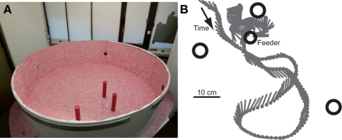
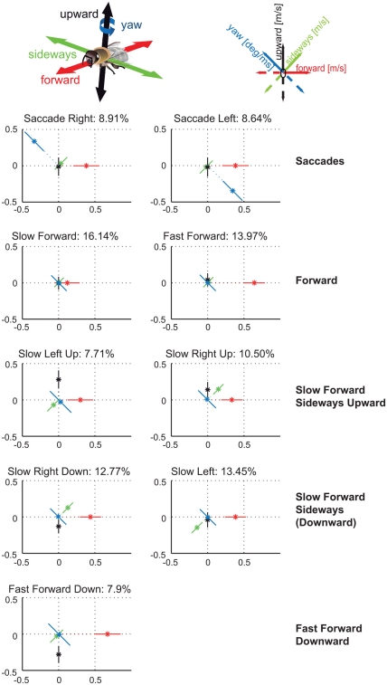
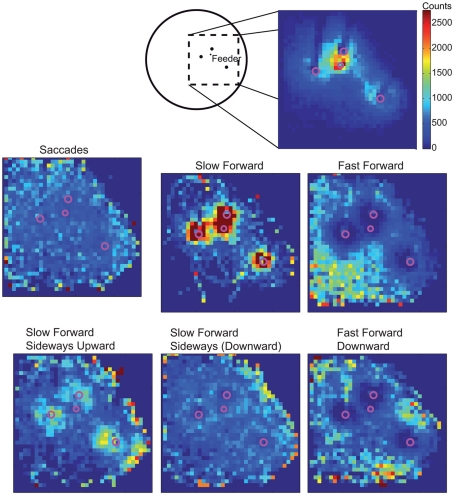
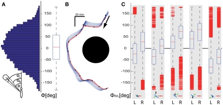
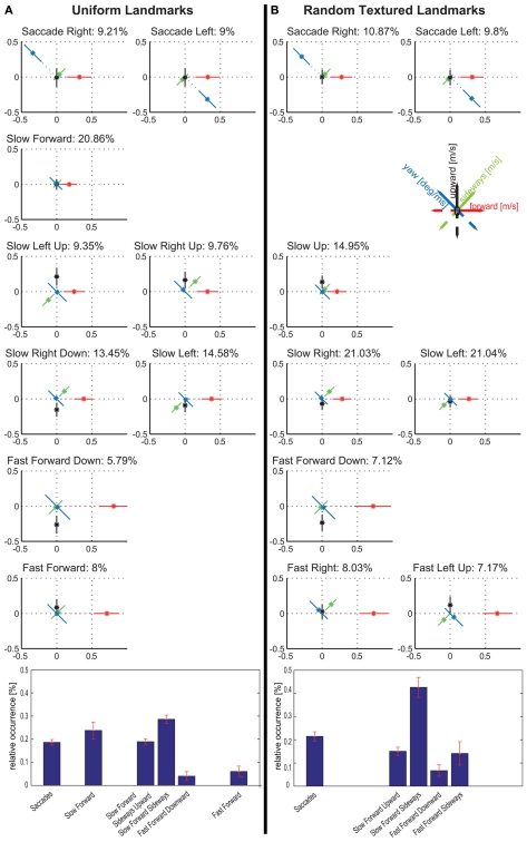
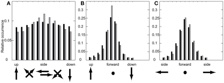
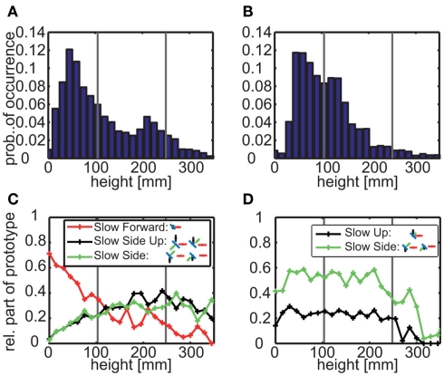
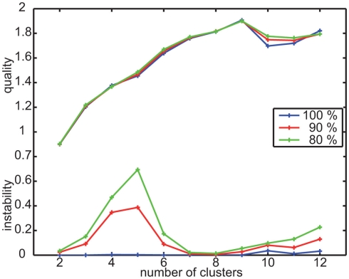
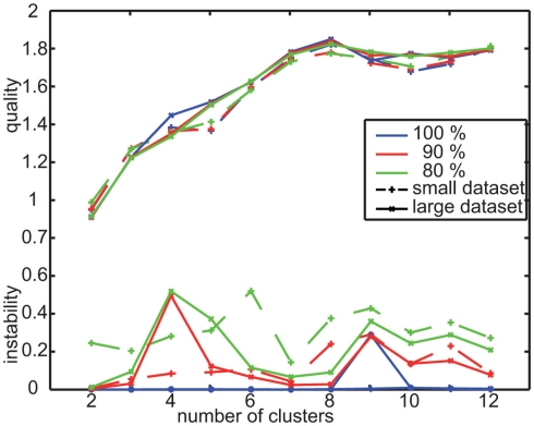
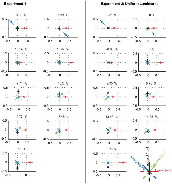
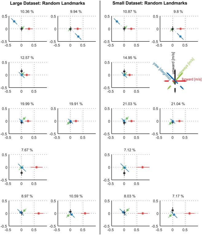
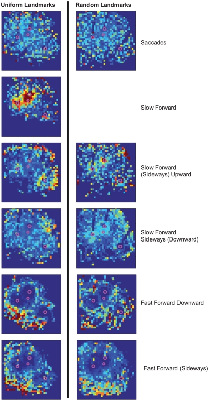
Honeybees use visual cues to relocate profitable food sources and their hive. What bees see while navigating, depends on the appearance of the cues, the bee's current position, orientation, and movement relative to them. Here we analyze the detailed flight behavior during the localization of a goal surrounded by cylinders that are characterized either by a high contrast in luminance and texture or by mostly motion contrast relative to the background. By relating flight behavior to the nature of the information available from these landmarks, we aim to identify behavioral strategies that facilitate the processing of visual information during goal localization. We decompose flight behavior into prototypical movements using clustering algorithms in order to reduce the behavioral complexity. The determined prototypical movements reflect the honeybee's saccadic flight pattern that largely separates rotational from translational movements. During phases of translational movements between fast saccadic rotations, the bees can gain information about the 3D layout of their environment from the translational optic flow. The prototypical movements reveal the prominent role of sideways and up- or downward movements, which can help bees to gather information about objects, particularly in the frontal visual field. We find that the occurrence of specific prototypes depends on the bees' distance from the landmarks and the feeder and that changing the texture of the landmarks evokes different prototypical movements. The adaptive use of different behavioral prototypes shapes the visual input and can facilitate information processing in the bees' visual system during local navigation.

Keywords: classification of behavior; honeybee local navigation; prototypical movements.

Figure 1

(A) Flight arena with the three landmarks. The upper cover of the arena made of cloth is not shown. (B) Sample trajectory as seen from above. The position (gray dot) and orientation (gray line) of the bee are shown every 24 ms. The locations of the three landmarks (big open circles) and the feeder (smaller open circle) are indicated.

Figure 2

Nine velocity prototypes for experiment 1 in (meter per second) and (degree per millisecond), respectively. Each prototype is depicted as star plot containing the four velocity components drawn onto color coded lines equally dividing the drawing plane. For each line the distance of the dot from the center determines the absolute value of the corresponding velocity component, the error bars visualize the SD of this value. Whether the value is positive or negative determines at which part of the line relative to zero point the value is plotted. Percentage of data points assigned to the individual prototypes determines the relative occurrence of each prototype. For detailed description, see text.

Figure 3

Sketch of the top-view of the arena and the area around the landmarks and the feeder that is covered by cameras for recording the trajectories. Spatial distribution of all analyzed trajectory points in 2D (irrespective of the height above the arena floor). Area is divided into 30 mm × 30 mm large cells and the absolute number of trajectory points assigned to one cell is visualized. C: spatial probabilities of occurrence of the nine velocity prototypes combined to six classes for better visualization. For each class of velocity prototypes’ absolute occurrences are counted within the 30-mm × 30-mm cells and, firstly, normalized with the overall spatial distribution. Finally, each distribution is normalized to sum up to 1 and, therefore, corresponds to the spatial probability of occurrence of this prototype class. The same color code is used for all distributions.

Figure 4

Analysis of the angle Φ between the orientation of the bee and the direction of the landmark center, which approximates the viewing angle of the landmark. (A) Distribution and corresponding boxplot indicating the median and quartiles and the range of the viewing angles Φ to the center of the landmarks for all trajectory points with the bee closer than 100 mm from the center of the nearest landmark. (B) Example trajectory of a flight near to the landmark as seen from above. The position of the bee’s center of mass (dot) and its orientation (line) are shown every 8 ms. (C) Angles of view of the right and left edge of the nearest landmark, (indicated by R and L below the respective subplot) for the same data as analyzed in (A) in dependence on the corresponding prototypical movement. The median, quartiles, and range of the data are shown. Outliers are displayed as short horizontal bars; data points are drawn as outliers if they are larger than 1.5 of the distance between the 25th and 75th percentiles. This corresponds to ∼±2.7 ( and 99.3 coverage if the data are normally distributed. Only data corresponding to the prototypes providing slow forward velocities are depicted underneath the subplots because they predominantly occur near to the landmarks; prototypes are depicted in the format as explained in Figure 2.

Figure 5

Comparison between velocity prototypes resulting from tests with uniformly red coloured (A) and randomly textured (B) landmarks for experiment 2. Bar diagram shows the relative occurrences for prototype classes. Error bars show the mean error of the mean value of the occurrence data for the individual bees. For detailed description, see text.

Figure 6

Probability distributions of velocity component combinations measured as histograms of the occurrence of relations between two components. Dark: uniform landmarks, gray: random landmarks. (A) Upward/sideways/downward velocity, (B) upward/forward/downward, (C) left/forward/right.

Figure 7

(A,B) Height probability distributions for all trajectory points that are near to the uniform (A) or randomly textured (B) landmarks (distance < 100 mm). The data sets contain 23,891 points out of 84,374 (corresponding to 191 s) for uniform landmarks and 15,877 points (corresponding to 127 s) out of 65,004 for randomly textured landmarks. Gray vertical lines mark the height of the feeder (105 mm) and the landmarks (250 mm), respectively. (C,D) Relative part of different prototypes depending on the height near to the uniform (C) or randomly textured (D) landmarks. The saccadic prototypes are not depicted here, because they are rather uniformly distributed within the flight arena. The fast forward prototypes do not play a role near to the landmarks at all.

Figure A1

Quality and instability criterion for clustering the velocity data of experiment 1. Determine suitable number of clusters by minimizing instability and maximizing quality to be nine.

Figure A2

Quality and instability for two data sets recorded with randomly textured landmarks. Small data set contains the 41 flights of the nine bees that were also tested with uniform landmarks. Large dataset is extended by additional data and contains 79 flights from 16 bees at all.

Figure A3

Comparison between prototypes resulting from clustering the data of experiment 1 and the data within the same condition (three uniformly red colored landmarks) of experiment 2. Clustering the independent data set of experiment 2 leads again to nine clusters providing the maximal quality and being sufficiently stable (data not shown). The resulting velocity prototypes are similar to those obtained in experiment 1. There are only quantitative differences in the relative occurrences of the velocity prototypes between the data sets which, however, do not affect our conclusions. The spatial probability distributions of occurrence of the different prototypes are also similar between the two experiments (Figure A5).

Figure A4

Comparison between prototypes resulting from all available 79 flights for the random texture condition (left) and the 41 flights of the nine individuals that were also tested with the uniformly red landmarks (right). Again, there are no qualitative differences within the prototypes themselves, but in details of the relative occurrences.

Figure A5

Spatial distributions of occurrence probabilities of the prototypes of experiment 2. There are no characteristic differences in the spatial distributions of occurrences of the prototypes in dependence on the landmark texture. The saccadic prototypes are rather equally distributed under both landmark conditions. During the intersaccadic intervals, the prototypical forward velocity mainly determines the probability distributions. Increasing forward velocity shifts the probability of occurrence to areas of larger distance to the landmarks. For the random landmarks, there is no prototype as concentrated near to the landmarks as for the uniform landmarks, because this Slow Forward prototype does not occur for randomly textured landmarks. Instead, the existing prototypes providing slow forward velocities occur more often very close to the landmarks than the remaining prototypes for the uniform landmarks.

References

1. Baddeley B., Philippides A., Graham P., Hempel de Ibarra N., Collett T., Husbands P. (2009). What can be learnt from analysing insect orientation flights using probabilistic SLAM? Biol. Cybern. 101, 169–18210.1007/s00422-009-0327-4 - DOI - PubMed
1. Baird E., Srinivasan M. V., Zhang S., Lamont R., Cowling A. (2006). “Visual control of flight speed and height in the honeybee,” in From Animals to Animats, Vol. 4095, ed. Nolfi S. (Berlin: Springer; ), 40–51
1. Boeddeker N., Dittmar L., Stürzl W., Egelhaaf M. (2010). The fine structure of honeybee head and body movements in a homing task. Proc. Biol. Sci. 277, 1899–190610.1098/rspb.2009.1928 - DOI - PMC - PubMed
1. Braun E., Geurten B., Egelhaaf M. (2010). Identifying prototypical components in behaviour using clustering algorithms. PLoS ONE 5, e9361.10.1371/journal.pone.0009361 - DOI - PMC - PubMed
1. Cartwright B., Collett T. (1983). Landmark learning in bees-experiments and models. J. Comp. Physiol. A 151, 521–54310.1007/BF00605469 - DOI
LinkOut - more resources