. 2012 Oct;33(2):227-55.
doi: 10.1007/s10827-012-0384-x. Epub 2012 Feb 4.

Uncovering spatial topology represented by rat hippocampal population neuronal codes

Affiliations

Uncovering spatial topology represented by rat hippocampal population neuronal codes

Zhe Chen et al. J Comput Neurosci. 2012 Oct.

Abstract

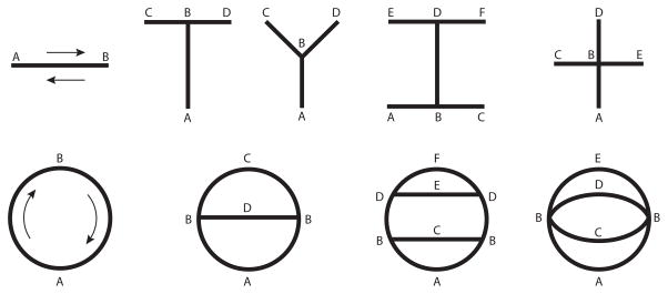
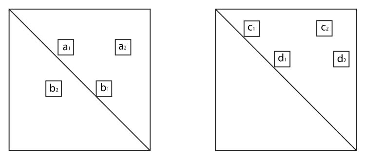
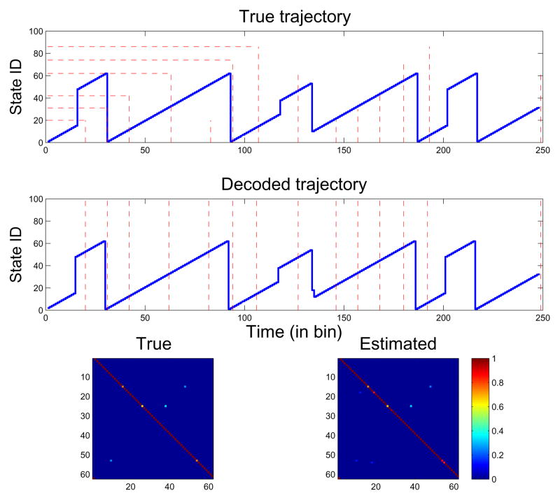
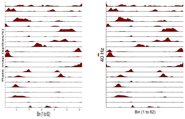
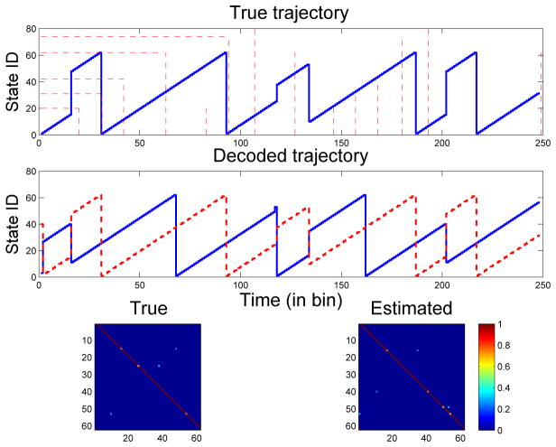
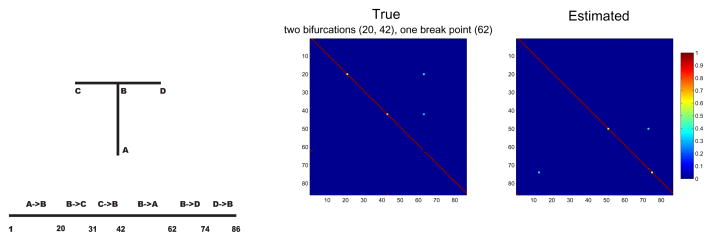
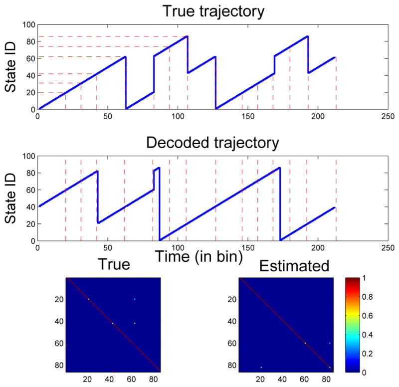
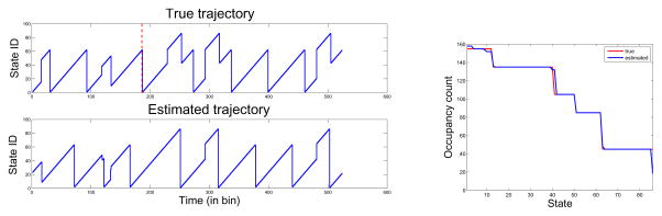
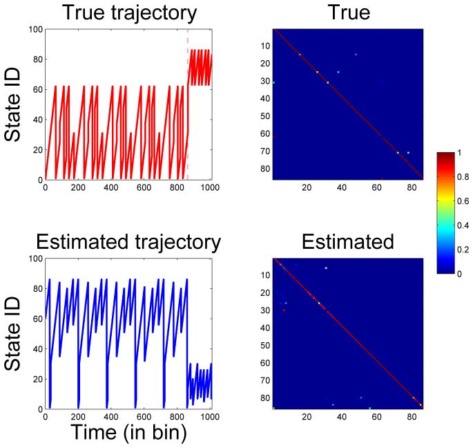
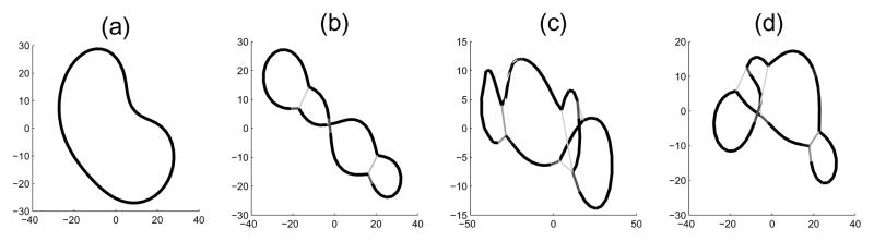
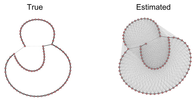
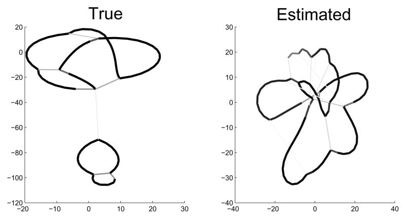
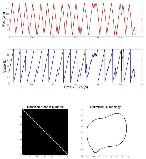
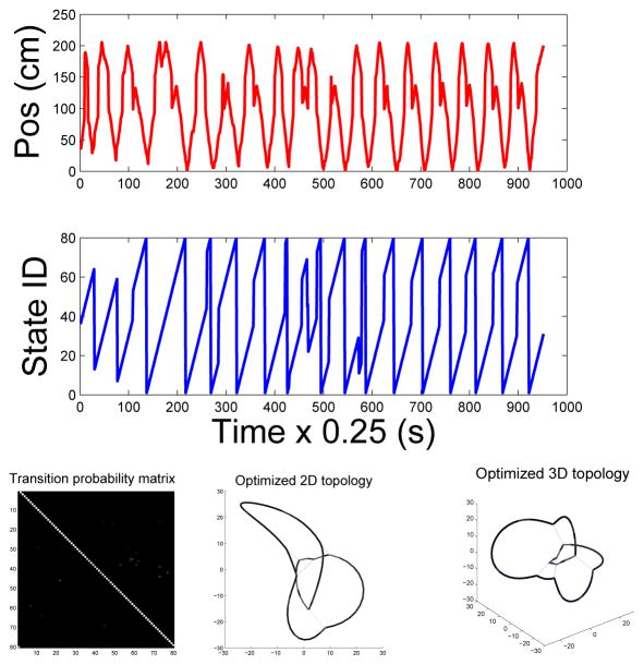
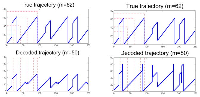
Hippocampal population codes play an important role in representation of spatial environment and spatial navigation. Uncovering the internal representation of hippocampal population codes will help understand neural mechanisms of the hippocampus. For instance, uncovering the patterns represented by rat hippocampus (CA1) pyramidal cells during periods of either navigation or sleep has been an active research topic over the past decades. However, previous approaches to analyze or decode firing patterns of population neurons all assume the knowledge of the place fields, which are estimated from training data a priori. The question still remains unclear how can we extract information from population neuronal responses either without a priori knowledge or in the presence of finite sampling constraint. Finding the answer to this question would leverage our ability to examine the population neuronal codes under different experimental conditions. Using rat hippocampus as a model system, we attempt to uncover the hidden "spatial topology" represented by the hippocampal population codes. We develop a hidden Markov model (HMM) and a variational Bayesian (VB) inference algorithm to achieve this computational goal, and we apply the analysis to extensive simulation and experimental data. Our empirical results show promising direction for discovering structural patterns of ensemble spike activity during periods of active navigation. This study would also provide useful insights for future exploratory data analysis of population neuronal codes during periods of sleep.


Figures

Fig. 1
Fig. 1
Examples of experimental space topology explored by animal (For left to right: linear track, T-maze, Y-maze, H-maze, cross maze). The arrow indicates the traveling direction. The first row shows the physical shape of the track, and the second row shows the corresponding (equivalent) topology by considering the bidirectional factor. Note that the T-maze and Y-maze have two bifurcation points (each with 2 possible choices), the H-maze has four bifurcation points (each with 2 possible choices), and the cross-maze has two bifurcation points (each with 3 possible choices).
Fig. 2
Fig. 2
Cartoon illustration for comparing two matrix-rows that have two dominant off-diagonal elements, where a1, b1, c1, d1 are the one-column-right-shifted diagonal elements (i.e., column index = row index + 1).
Fig. 3
Fig. 3
One illustrated estimation result from the linear track (Simulation 1-2): the true trajectory in one lap (top) and the corresponding estimated trajectory (middle). State 1–31 represents the left-to-right positions inside the linear track, and state 32–62 represents right-to-left positions inside the track. The color-coded true (bottom left) and estimated (bottom right) transition matrices are qualitatively and quantitatively similar. Note that the transition matrix has a shifted-diagonal structure. Quantitative indices: D1 = 0.1333, D2(2) = 0.0407, D2(3) = 0.0479.
Fig. 4
Fig. 4
The simulated (left) and estimated (right) tuning curves of 21 neurons from the same result shown in Fig. 3 (Simulation 1-2). The full length of the vertical bar marks the firing rate scale of 40 Hz.
Fig. 5
Fig. 5
In comparison with the results illustrated in Fig. 3, another correct estimation result from the trajectory in a linear track (Simulation 1–2). Note that the the raw (top panel) and remapped (second panel, dashed line) state trajectories will become nearly identical upon state ID remapping (using the following ID map: [1:25]→[38:62], [26:62]→[1:37]). Also note that the true (bottom left) and estimated (bottom right) transition matrices will become nearly identical upon state ID remapping. Quantitative indices: D1 = 0.1333, D2(2) = 0.0560, D2(3) = 0.093.
Fig. 6
Fig. 6
Scatter plots of statistics of D1, D2(2), and free energy F. Statistics are obtained from 50 independent Monte Carlo simulations (Simulation 1-2).
Fig. 7
Fig. 7
Left: illustration of linearization of a simulated T-maze. Due to the bidirectional factor of the place field, a total of 43×2 = 86 states represents the 43 bins. Linearized bin assignment: AB: 1:20, BC: 21:31, CB: 32:42, BA: 43:62, BD: 63:74, DB: 75:86. One illustrated result from the simulated T-maze (Simulation 2-1): color-coded true (middle) and estimated (right) transition probability matrices, and D2(2) = 0.015. The comparison of the true and estimated trajectories are not shown here.
Fig. 8
Fig. 8
One illustrated snapshot from the simulated T-maze (Simulation 2-2). Top: comparison of the true and estimated trajectories. Bottom: comparison of the true (left) and estimated transition matrices (right). Quantitative indices: D1 = 0, D2(2) = 0.024, D2(3) = 0.038.
Fig. 9
Fig. 9
One illustrated snapshot from two combined environments (Simulation 3-1): the comparison of the snapshots of the true (left top) and estimated (left bottom) trajectories, with the transition marked by a dashed line. In this case, two environments have overlapping regions. From the true and estimated state trajectories, we can compare the statistics of the state occupancy time (right) and obtain D1 = 0.783.
Fig. 10
Fig. 10
One illustrated result from two combined environments (Simulation 3-2): the comparison of the snapshots of the true (top left) and estimated (bottom left) trajectories. Note that two environments have no overlapping region, the one-time transition between A and B (31 → 63) is marked by a dashed line. Linear track A has state ID 1-31 (forward direction) and 32–62 (reverse direction); linear track B has state ID 63–74 (forward direction) and 75–86 (reverse direction). Quantitative indices: D1 = 3.04, D2(2) = 0.313, D2(3) = 0.445.
Fig. 11
Fig. 11
(a) The graph inferred from the estimated transition matrix from a simulated linear track without behavioral turns (Simulation 1-1, m = 62). (b–d): the graphs inferred from a simulated linear track with behavioral turns (Simulation 1-2, m = 62): from the true transition matrix (b), the estimated transition matrix (c) and the estimated transition matrix followed by 0.05 thresholding (d).
Fig. 12
Fig. 12
The graphs inferred from the true estimation matrix (left) and the estimated transition matrix without thresholding (right) in a simulated T-maze (Simulation 2-2, m = 86). The nodes represent the states, and the edges represent the strengths between the nodes. Notice the similar spatial topology between these two graphs.
Fig. 13
Fig. 13
The graphs inferred from the true transition matrix (left) and the estimated transition matrix with 0.01 thresholding (right) in Simulation 3-2 (m = 86).
Fig. 14
Fig. 14
One illustrated estimation result from the experimental linear track (m = 60): True position during the run period (top panel) and the decoded state sequence (middle panel). The estimated transition probability matrix (bottom left) and the inferred 2D graph (bottom right) are also shown. Note that there are three weak edges or shortcuts appended to the well-connected closed-loop.
Fig. 15
Fig. 15
One illustrated estimation result from the experimental T-maze (m = 80): True position during run period (top panel) and the decoded state sequence (middle panel). The estimated transition probability matrix (bottom left) and the inferred 2D (bottom middle) and 3D graphs (bottom right) are also shown. The 3D graph is simply another perspective to visualize the topological graph.
Fig. 16
Fig. 16
Illustration of the estimated trajectory where the model size mismatch (Simulation 1-2). Underestimation (left): m = 50, D1 = 8, D2(2) = 0.087, D2(3) = 0.093. Overestimation (right): m = 80, D1 = 4, D2(2) = 0.017, D2(3) = 0.182.
Fig. 17
Fig. 17
Illustration of the distribution statistics of the converged free energy value based on independent random initializations. In each setup (from Simulation 1-2), 100 Monte Carlo experiments are conducted. As expected, when the selected model order matches the true model size (m = 62), a higher free energy value is typically achieved.
Fig. 18
Fig. 18
Illustration of the estimated transition matrix in the presence of dummy state (left) and the inferred graph (right). The results are obtained from the experimental linear track data (using m = 60). Note that in the left panel, the non-sparse pattern of the 61st column implies frequent stop behavior from various spatial locations. Also note that in the right panel, the graph is drawn excluding the dummy state (i.e., based on the 60 × 60 submatrix of P), which gives rise to a spatial topology without the closed loop.
Fig. 19
Fig. 19
Illustration of the algorithmic convergence and stability (Simulation 2-2). At different stages (1st and 3rd iterations, and final convergence), the free energy (top row), the estimated state transition matrix (middle row), and the tuning curve of one neuron (bottom row) are shown.

Similar articles

Cited by

References

    1. Amari S, Ozeki T, Park HY. Learning and inference in hierarchical models with singularities. Systems and Computers in Japan. 2003;34(7):34–42.
    1. Baum LE, Petrie T, Soules G, Weiss N. A maximization technique occurring in the statistical analysis of probabilistic functions of Markov chains. Annals of Mathematical Statistics. 1970;41(1):164–171.
    1. Beal MJ, Ghahramani Z, Rasmussen CE. Advances in Neural Information Processing Systems. MIT Press; 2002. The infinite hidden Markov model; p. 14.
    1. Beal MJ. PhD Thesis. Gatsby Computational Neuroscience Unit, University College London; 2003. Variational algorithms for approximate Bayesian inference.
    1. Bellman R. Dynamic Programming. Princeton University Press; Boston: 1957.

Publication types

LinkOut - more resources