. 2012 May 8;109(19):E1134-42.
doi: 10.1073/pnas.1116619109. Epub 2012 Feb 13.

Global climate evolution during the last deglaciation

Affiliations

Global climate evolution during the last deglaciation

Peter U Clark et al. Proc Natl Acad Sci U S A. .

Abstract

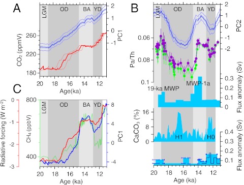
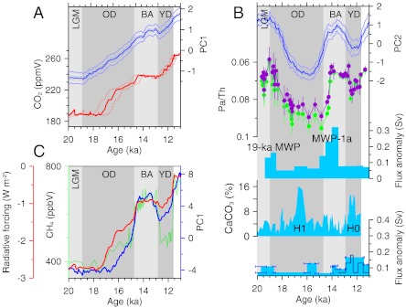
Deciphering the evolution of global climate from the end of the Last Glacial Maximum approximately 19 ka to the early Holocene 11 ka presents an outstanding opportunity for understanding the transient response of Earth's climate system to external and internal forcings. During this interval of global warming, the decay of ice sheets caused global mean sea level to rise by approximately 80 m; terrestrial and marine ecosystems experienced large disturbances and range shifts; perturbations to the carbon cycle resulted in a net release of the greenhouse gases CO(2) and CH(4) to the atmosphere; and changes in atmosphere and ocean circulation affected the global distribution and fluxes of water and heat. Here we summarize a major effort by the paleoclimate research community to characterize these changes through the development of well-dated, high-resolution records of the deep and intermediate ocean as well as surface climate. Our synthesis indicates that the superposition of two modes explains much of the variability in regional and global climate during the last deglaciation, with a strong association between the first mode and variations in greenhouse gases, and between the second mode and variations in the Atlantic meridional overturning circulation.


Conflict of interest statement

The authors declare no conflict of interest.

Figures

Fig. 1.
Fig. 1.
(A) Climate simulation of the Last Glacial Maximum 21,000 y ago using the National Center for Atmospheric Research Community Climate System Model, version 3.0 (141). Sea-surface temperatures are anomalies relative to the control climate. Also shown are continental ice sheets (1,000-m contours) (149) and leaf-area index simulated by the model (scale bar shown). (B) Same as A except for 11 ka.
Fig. 2.
Fig. 2.
Climate records and forcings during the last deglaciation. The oxygen-isotope (δ18O) records from Greenland Ice Sheet Project Two (GISP2) (150) (dark-blue line) and Greenland Ice Core Project (GRIP) (151) (light-blue line) Greenland ice cores shown in (A) (placed on the GICC05 timescale; ref. 57) document millennial-scale events that correspond to those first identified in northern European floral and pollen records. LGM, Last Glacial Maximum; OD, Oldest Dryas; BA, Bølling–Allerød; ACR, Antarctic Cold Reversal; YD, Younger Dryas. (B) Oxygen-isotope (δ18O) record from European Project for Ice Coring in Antarctica (EPICA) Dronning Maud Land (152) (dark-green line) and deuterium (δD) record from Dome C (45) (light-green line) Antarctic ice cores, placed on a common timescale (2). (C) Midmonth insolation at 65°N for July (orange line) and at 65°S for January (light-blue line) (153). (D) The combined radiative forcing (red line) from CO2 (blue dashed line), CH4 (green dashed line), and N2O (purple dashed line) relative to preindustrial levels. CO2 is from EPICA Dome C ice core (1) on Greenland Ice Core Chronology 05 (GICC05) timescale from ref. , CH4 is from GRIP ice core (154) on the GICC05 timescale, and N2O is from EPICA Dome C (155) and GRIP (156) ice cores on the GICC05 timescale. Greenhouse gas concentrations were converted to radiative forcings using the simplified expressions in ref. . The CH4 radiative forcing was multiplied by 1.4 to account for its greater efficacy relative to CO2 (158). (E) Relative sea-level data from Bonaparte Gulf (green crosses) (159), Barbados (gray and dark-blue triangles) (160), New Guinea (light-blue triangles) (161, 162), Sunda Shelf (purple crosses) (163), and Tahiti (green triangles) (164). Also shown is eustatic sea level (gray line) (165). (F) Rate of change of area of Laurentide Ice Sheet (LIS) (166) and Scandinavian Ice Sheet (SIS) (SI Appendix). (G) Freshwater flux to the global oceans derived from eustatic sea level in E. (H) Record of ice-rafted detrital carbonate from North Atlantic core VM23-81 identifying times of Heinrich events 1 and 0 (167). (I) Freshwater flux associated with routing of continental runoff through the St. Lawrence and Hudson rivers (filled blue time series) with age uncertainties (168). Also shown is time series of runoff through the St. Lawrence River during the Younger Dryas (solid blue line) (142).
Fig. 3.
Fig. 3.
(A) Principal component (PC) 1 based on all of the SST records (solid blue line). PC1s based only on alkenone (dashed light-blue line) and Mg/Ca records (dashed orange line) are also shown. The percentage of variance explained by PC1 is 49%, by PC1 (Mg/Ca) is 59%, and by PC1 (formula image) is 64%. (B) PC2 based on all of the SST records (solid blue line). PC2s based only on alkenone (dashed light-blue line) and Mg/Ca records (dashed orange line) are also shown. The percentage of variance explained by PC2 is 29%, by PC2 (Mg/Ca) is 13%, and by PC2 (formula image
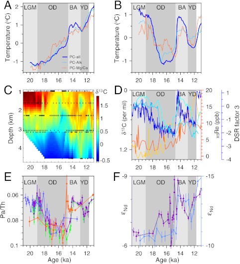
) is 15%. (C) Temporal evolution of δ13C in the North Atlantic basin reconstructed from data shown by black diamonds based on a depth transect of six marine cores (, , , –171). (D) Proxy records of intermediate-depth waters from the Arabian Sea and Pacific Ocean. Cyan line is δ13C record from the Arabian Sea (20), sky blue line is five-point running average of δ13C record from the SW Pacific Ocean (19), blue line is diffuse spectral reflectance (factor 3 loading) (a proxy of organic carbon) from the North Pacific (24), yellow and orange lines are records of excess Re (a proxy of dissolved oxygen) from the southeast Pacific (21). (E) Pa/Th records from the North Atlantic Ocean (27, 28, 172). (F) ϵNd records from the North Atlantic (14) (blue line) and south Atlantic (173) (purple line). Abbreviations are as in Fig. 2.
Fig. 4.
Fig. 4.
Regional and global principal components (PCs) for temperature (T) and precipitation (P) based on records shown on map in lower left. Red dots on map indicate sites used to constrain ocean sea-surface temperatures, yellow dots constrain continental temperatures, and blue dots constrain continental precipitation. PC1s are shown as blue lines, PC2s as red lines. We used a Monte Carlo procedure to derive error bars (1σ) for the principal components which reflect uncertainties in the proxy records. All records were standardized to zero mean and unit variance prior to calculating EOFs, which is necessary because the records are based on various proxies and thus have widely ranging variances in their original units (SI Appendix).
Fig. 5.
Fig. 5.
(A) Comparison of the global temperature PC1 (blue line, with confidence intervals showing results of jackknifing procedure for 68% and 95% of records removed) with record of atmospheric CO2 from EPICA Dome C ice core (red line with age uncertainty) (1) on revised timescale from ref. . (B) Comparison of the global temperature PC2 (blue line, with confidence intervals showing results of jackknifing procedure for 68% and 95% of records removed) with Pa/Th record (a proxy for Atlantic meridional overturning circulation) (27) (green and purple symbols). Also shown are freshwater fluxes from ice-sheet meltwater, Heinrich events, and routing events (Fig. 2). (C) Comparison of the global precipitation PC1 (blue line) with record of methane (green line) and radiative forcing from greenhouse gases (red line) (see Fig. 2D). Abbreviations are as in Fig. 2.
Fig. P1.
Fig. P1.
(A) Comparison of the global temperature PC1 (blue line, with confidence intervals showing results of jackknifing procedure for 68% and 95% of records removed) with record of atmospheric CO2 from European Project for Ice Coring in Antarctica Dome C ice core (red line with age uncertainty) (4) on revised timescale from ref. . (B) Comparison of the global temperature PC2 (blue line, with confidence intervals showing results of jackknifing procedure for 68% and 95% of records removed) with Pa/Th record (a proxy for Atlantic meridional overturning circulation) (3) (green and purple symbols). Also shown are freshwater fluxes from ice-sheet meltwater, Heinrich events, and routing events. (C) Comparison of the global precipitation PC1 (blue line) with record of methane (green line) and radiative forcing from greenhouse gases (red line). OD, Oldest Dryas; BA, Bølling—Allerød; YD, Younger Dryas; MWP, meltwater pulse.

Similar articles

Cited by

References

    1. Monnin E, et al. Atmospheric CO2 concentrations over the last glacial termination. Science. 2001;291:112–114. - PubMed
    1. Lemieux-Dudon B, et al. Consistent dating for Antarctic and Greenland ice cores. Quat Sci Rev. 2010;29:8–20.
    1. Brook EJ, Harder S, Severinghaus J, Steig EJ, Sucher CM. On the origin and timing of rapid changes in atmospheric methane during the last glacial period. Global Biogeochem Cycles. 2000;14:559–571.
    1. Schilt A, et al. Glacial-interglacial and millennial-scale variations in the atmospheric nitrous oxide concentration during the last 800,000 years. Quat Sci Rev. 2010;29:182–192.
    1. Broecker WS. Thermohaline circulation, the Achilles heel of our climate system: Will man-made CO2 upset the current balance. Science. 1997;278:1582–1588. - PubMed

Publication types