. 2012;7(2):e30024.
doi: 10.1371/journal.pone.0030024. Epub 2012 Feb 20.

Single Molecule Analysis Research Tool (SMART): an integrated approach for analyzing single molecule data

Affiliations

Single Molecule Analysis Research Tool (SMART): an integrated approach for analyzing single molecule data

Max Greenfeld et al. PLoS One. 2012.

Abstract

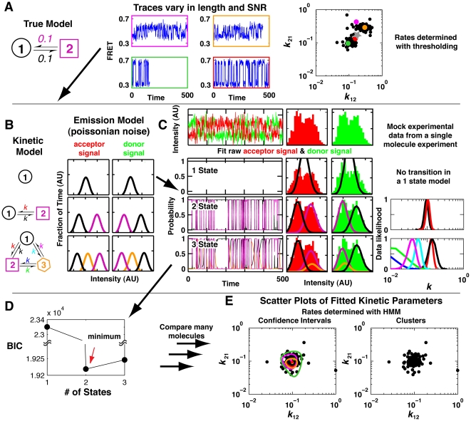
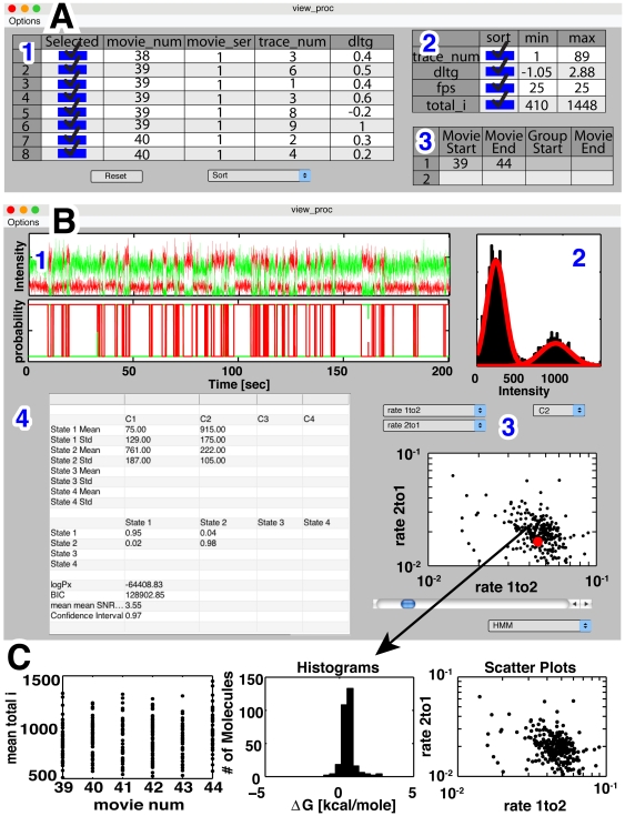
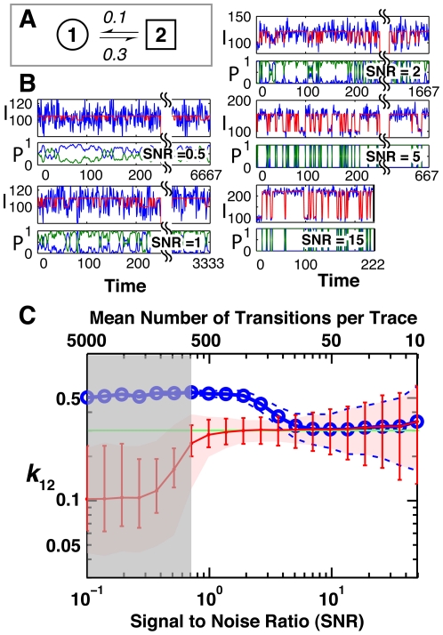
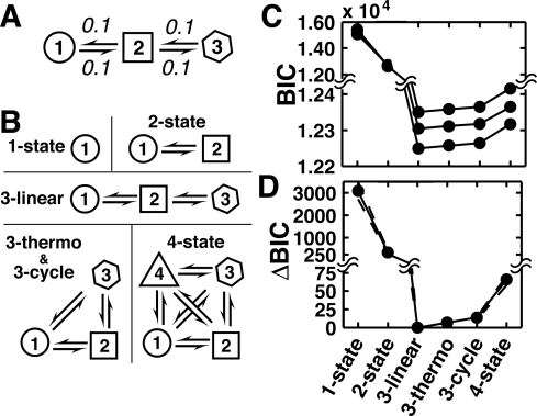
Single molecule studies have expanded rapidly over the past decade and have the ability to provide an unprecedented level of understanding of biological systems. A common challenge upon introduction of novel, data-rich approaches is the management, processing, and analysis of the complex data sets that are generated. We provide a standardized approach for analyzing these data in the freely available software package SMART: Single Molecule Analysis Research Tool. SMART provides a format for organizing and easily accessing single molecule data, a general hidden Markov modeling algorithm for fitting an array of possible models specified by the user, a standardized data structure and graphical user interfaces to streamline the analysis and visualization of data. This approach guides experimental design, facilitating acquisition of the maximal information from single molecule experiments. SMART also provides a standardized format to allow dissemination of single molecule data and transparency in the analysis of reported data.


Conflict of interest statement

Competing Interests: The authors have declared that no competing interests exist.

Figures

Figure 1
Figure 1. Workflow for SMART analysis of single molecule data.
In a typical analysis of single molecule data the distribution of rate constants determined from a simple two-state system can appear heterogeneous because of uncertainties that arise from variation in trace length and SNR. SMART addresses these limitations. Part A (left) shows a simple model used to generate 200 simulated traces, with SNR's of either 4 or 12 and trace lengths determined by a photobleaching model (see Methods). Four representative traces are shown, and the time constants for these four molecules (colors) and each of the other simulated molecules (black) determined by threshold analysis are plotted on the right. The gray star represents the inferred transition rate assuming all the molecules arose from the same population of molecules. Panels B–E show analysis of the single molecule FRET data from Panel A subject to SMART analysis. The analysis is shown for one molecule, and the data for all molecules are compared in Panel E. (B) The user specifies a set of kinetic and emission models to be fit to the observed trace. (C) Traces are analyzed individually. The donor (green) and acceptor (red) intensities are plotted as a function of time and are used directly in the fits. The cumulative histograms for the intensity of each are plotted on the right and are fit during the analysis. Fits of the models to the data are shown for the one-, two-, and three-state models of Panel B. State occupancy probabilities are shown on the left, fitted emission distributions are depicted in the middle, and the inferred transition rates between states (k xy), and normalized likelihood values (confidence intervals) are plotted on the right (colors depict rate constants for different transitions). SMART is able to calculate confidence intervals for each of the fitted parameters. (D) The Bayesian information criterion (BIC) is used to select a model that best balances goodness of fit and the number of free parameters. The fit with the lowest Bayesian information criteria has the optimal fit. (E) Summary of data from steps (B) and (C) for the entire population of 200 molecules. The plots show different representations of uncertainties, with confidence intervals on the left (shown explicitly only for the colored traces from Panel A) and as clusters on the right (one cluster is shown). The molecules that segregated into two apparent classes by thresholding have overlapping confidence intervals (left) and fall in the same cluster (right) and thus do not provide evidence for distinct populations of molecules.
Figure 2
Figure 2. Highlights of SMART, an integrated data analysis tool that combines general HMM algorithms with graphical user interfaces to allow data to be visualized and rapidly analyzed.
(A) Molecules can be selected on the basis of experiment type and/or fitted parameters: (A1) Fitted parameters can be inspected and molecules manually selected in tabular form. (A2) Molecules can be selected based on a user-specified range of experimental or fit values. (A3) Molecules can be selected by a user-defined experiment number or numbers. (B) Interactive data viewing environment allows inspection and plotting of raw data and fitted model parameters: (B1) A raw trace and the estimated state occupancies. (B2) Cumulative emission distributions and fitted emissions model. (User chooses which channel is shown.) (B3) Scatter plot of all molecules of the user-specified group. The red dot indicates the molecule that is summarized in B1, B2, and B4. (B4) Fitted model parameters for the indicated molecule displayed in tabular form. (C) The environment (B3) allows the rapid generation of data summaries for the specified molecules and displays them graphically; three additional data summary graph formats are shown in Part C.
Figure 3
Figure 3. Comparison of HMM and thresholding for identifying the true rate constants from traces varying over a range of SNRs with trace length (not shown) inversely proportional to SNR to account for photobleaching in smFRET experiments.
(A) The two-state kinetic model used in simulating traces over a range of SNRs. (B) Anecdotal traces at five different SNRs, simulated emissions (see Methods) are shown in blue and the true state being occupied is shown in red. Two-state HMM fits are shown below the simulated traces. The blue line indicates the probability of being in state 1 (low intensity) the green line indicates the probability of being in state 2 (high intensity). I and P on the ordinate of the traces indicate intensity and probability, respectively, for each SNR. (C) The average inferred rate constants obtained using thresholding (blue) and HMM modeling (red) as a function of the SNR. The true value, represented by the horizontal green line, is 0.3 (Panel A). The dotted blue line and red swath represent the region that bounds 90% of the determined rate constants from the 500 simulated traces analyzed for HMM and threshold fits, respectively. The mean number of transitions per trace is indicated at the top of the graph. As the difference in signal means for true transitions becomes negligible relative to the noise, the BIC indicates that a one-state fit provides the best fit to the data; this region is shown by the gray swath.
Figure 4
Figure 4. Testing the ability of the BIC to identify the true model.
(A) Three-state model used to generate mock traces. In this model, states 1 and 2 had emission properties identical to the states in Fig. 3A (also see Methods), and the equivalent of the SNR of 4 from that figure was used. State 3 was added with emission halfway between these states, resulting in an effective SNR between states of 2. (B) Simulated traces were fit to six different HMM models. The 3-thermo and 3-cycle models have identical topology but 3-thermo was fit using a constraint of thermodynamic closure (i.e., the rate constants determined will satisfy detailed balance) and therefore has one fewer fitted parameter than 3-cycle. (C) Plots of the BIC for the six different models. Three BICs for three example traces are shown in black. (D) Same data as in part C except that the difference between the 3-linear BIC (lowest in all cases) and the BIC for the other models is plotted. The solid black line indicates the mean of this difference for 1000 traces and the dashed lines indicate 90% confidence intervals.
Figure 5
Figure 5. Clustering algorithms to identify two non-exchanging populations of molecules.
(A) Traces with SNRs of 2, 5, 10 and 15 were generated from two non-exchanging pools of molecules (100 traces each) with one transition rate differing by two-fold. The traces were fit to two-state HMM models and subjected to clustering analysis in SMART. (B) Traces were fit with 1 to 4 clusters; the cluster size of the 2 and 3 cluster fits are shown while the 1 and 4 cluster fits are shown in Appendix S1. The black and green bars correspond to an individual cluster size at the indicated SNR; the bars corresponding to the third cluster in the third cluster fit is not visible due to its small size. (C) Scatter plots for two-cluster fits of the inferred rate constants. Black dots indicate the two inferred cluster centers, and blue dots indicate the true population centers.
Figure 6
Figure 6. Analysis of heterogeneity in smP4–P6 RNA with simulations and SMART clustering.
The smP4–P6 data and simulation analysis are from Greenfeld et al. . (A) Folding and unfolding rates of smP4–P6 (black) were analyzed by simulating two non-exchanging populations of molecules whose rate constants differ by two-fold (red). By this analysis 80% of the molecules are accounted for by the simulated data. (B) The inferred cluster size for fits of 1 to 5 clusters of the folding and unfolding rates of smP4–P6. (C) Color-coded smP4–P6 kinetics from the four-cluster fit. The two central clusters account for 90% of the molecules.

Similar articles

Cited by

References

    1. Roy R, Hohng S, Ha T. A practical guide to single-molecule FRET. Nat Methods. 2008;5:507–516. - PMC - PubMed
    1. Weiss S. Fluorescence spectroscopy of single biomolecules. Science. 1999;283:1676–1683. - PubMed
    1. Lu HP. Probing single-molecule protein conformational dynamics. Acc Chem Res. 2005;38:557–565. - PubMed
    1. Joo C, Balci H, Ishitsuka Y, Buranachai C, Ha T. Advances in single-molecule fluorescence methods for molecular biology. Annu Rev Biochem. 2008;77:51–76. - PubMed
    1. Ambrose WP, Goodwin PM, Jett JH, Van Orden A, Werner JH, et al. Single molecule fluorescence spectroscopy at ambient temperature. Chem Rev. 1999;99:2929–2956. - PubMed

Publication types