Efficient exact maximum a posteriori computation for bayesian SNP genotyping in polyploids

Abstract

The problem of genotyping polyploids is extremely important for the creation of genetic maps and assembly of complex plant genomes. Despite its significance, polyploid genotyping still remains largely unsolved and suffers from a lack of statistical formality. In this paper a graphical bayesian model for SNP genotyping data is introduced. This model can infer genotypes even when the ploidy of the population is unknown. We also introduce an algorithm for finding the exact maximum a posteriori genotype configuration with this model. This algorithm is implemented in a freely available web-based software package SuperMASSA. We demonstrate the utility, efficiency, and flexibility of the model and algorithm by applying them to two different platforms, each of which is applied to a polyploid data set: Illumina GoldenGate data from potato and Sequenom MassARRAY data from sugarcane. Our method achieves state-of-the-art performance on both data sets and can be trivially adapted to use models that utilize prior information about any platform or species.

Figure 1. Raw data.

The scatter plot of allele intensities for PotSNP034 (A), tetraploid, and SugSNP225 (B), which has an unknown ploidy.

Figure 2. A Graphical View of SNP Genotyping.

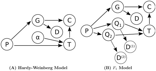
Two models for SNP genotyping are presented. Variables are shown as nodes and solid arrows depict dependencies between variables. The observed data depend on the genotypes of all individuals . In both models the distribution of genotypes is determined by the genotype configuration . Also, in both models the probability of a genotype distribution depends on , the distribution of genotypes in the population. Furthermore, both models use the same method to compute the probability of the data given the genotype configuration. Lastly, the possible genotypes depend on the ploidy . (A) In the Hardy-Weinberg model, the distribution of genotypes in the population is determined by one of the allele frequencies . (B) In the model, the distribution of genotypes in the population depends on the parent genotypes and . The dashed arrows and nodes ( and ) depict optional dependencies and variables; these variables and dependencies exist only when data from the parents is included.

Figure 3. Illustration of Exact Inference.

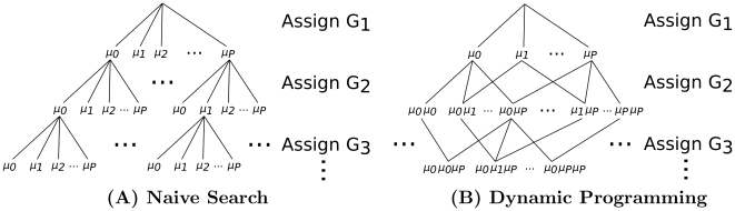
Exact MAP computation can be performed by enumerating all possible genotype configurations. Because each individual's genotype is among , searching through genotype configurations can be viewed as a tree in which each individual genotype assignment branches into separate outcomes. (A) A naive search progresses downward through the tree and chooses the series of genotype assignments that lead to the highest posterior probability. A naive branch and bound method derived from this tree bounds genotype configurations for which the prefix determines that all subsequent paths are poor. (B) A multinomial graph ( i.e. the subset graph of the power-set of G) merges outcomes that result in the same genotype counts . Multiple paths (from the top) can lead to any given set of genotype counts; therefore, dynamic programming is used. Given the layer above, each node can compute the most likely path from the top that leads to it. Once the most likely path and score are computed for each node in a layer, the next layer can progress. At the bottom layer, the node with the highest combined likelihood (computed via dynamic programming) and (the same for any path terminating at the node) maximizes the posterior probability. As in the naive tree, once all lower adjacent nodes in a subtree are provably suboptimal, then the subtree can be bounded. The dynamic programming approach is substantially more time space-efficient than the naive approach.

Figure 4. Illustration of a Suboptimal Genotype Configuration.

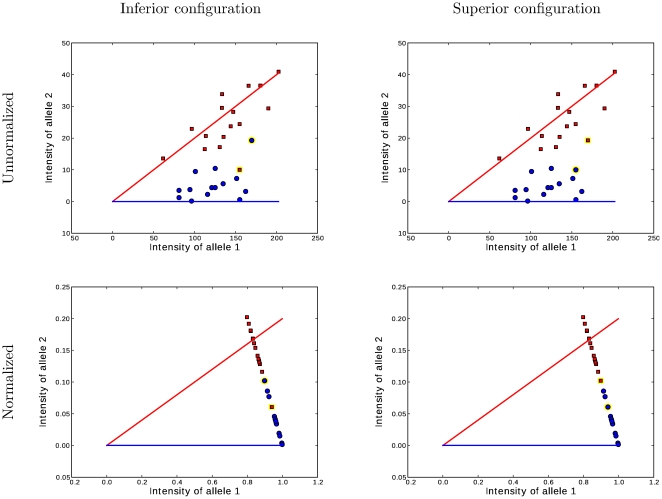
The essential motivation behind the geometric branch and bound is demonstrated. The top figure shows the original data and the bottom figure shows the data after being normalized to and within the likelihood function . The two figures on the left correspond to a suboptimal genotype configuration. In the figures on the right, a pair of “blue” and “red” points (highlighted) are switched to the opposite class. After swapping the categories, the numbers of individuals with each genotype do not change, but the total distance between these two points and their classes decreases. Decreasing this distance increases the likelihood while holding constant. Thus the joint probability . Because the MAP configuration cannot be improved by any such swaps, it must correspond to contiguous groups of class assignments along the normalized axis. Searching only the configurations that result in contiguous class assignments dramatically narrows the search space and makes inference computationally feasible where it wouldn't be with the dynamic programming branch and bound method.

Figure 5. Runtime of Exact MAP Computation with Dynamic Programming and Geometric Branch and Bound.

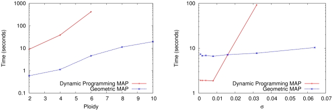
Both methods were run and timed while solving the same MAP inference problem. The y-axis plots the log of the runtime in seconds and the x-axis plots either the ploidy or the parameter . Both methods were implemented in Python and run on sugarcane locus SugSNP225 and timed using user time. Parental data was not used. For this data set, the optimal ploidy and values are . In the figure on the left, is held constant at and the ploidy is varied from 2 to 10. In the figure on the right, the ploidy is fixed at 10 and is doubled successively from to . In both figures, the dynamic programming branch and bound series is incomplete because the method was terminated after using more than 3 GB of RAM. In comparison, the geometric branch and bound method never used more than 50 MB. The growing gap between the methods indicates a superpolynomial speedup, especially when larger ploidies and larger values of are used. For very low values, the dynamic programming method is sometimes slightly faster due to decreased overhead.

Figure 6. SuperMASSA Output on Potato Loci.

For each potato locus (and the ploidy of the species analyzed), we show the output of SuperMASSA (using the –save_figures option). The first column shows the annotated scatter plot and the second column shows the theoretical distribution of genotypes in the population and the distribution of individuals assigned to each genotype. For both loci (in both the diploids and tetraploids), the genotype annotations are extremely close to the predicted angles for each assigned genotype and the genotype distributions are nearly identical to the theoretical distribution in a Hardy-Weinberg population using the MAP estimate for the parameter .

Figure 7. SuperMASSA Output on Sugarcane Loci.

For each sugarcane locus, we show the output of SuperMASSA (using the –save_figures option). The first column shows the annotated scatter plot and the second column shows the theoretical distribution of genotypes in the population and the distribution of individuals assigned to each genotype. In all three loci, the MAP configuration simultaneously finds the ploidy, a set of parents with that ploidy, and genotype assignments with tight clusters that produce nearly identical theoretical genotype distributions and genotype distributions.